Hyper Parameter Tuning

Hyper Parameter Tuning

• One way of searching for good hyper-parameters is by hand-tuning
• Another way of searching for good hyper-parameters is to divide each parameter’s valid range into evenly spaced values, and then simply have the computer try all combinations of parameter-values. This is called Grid Search.
• another way of searching for good hyper-parameters is by random search.
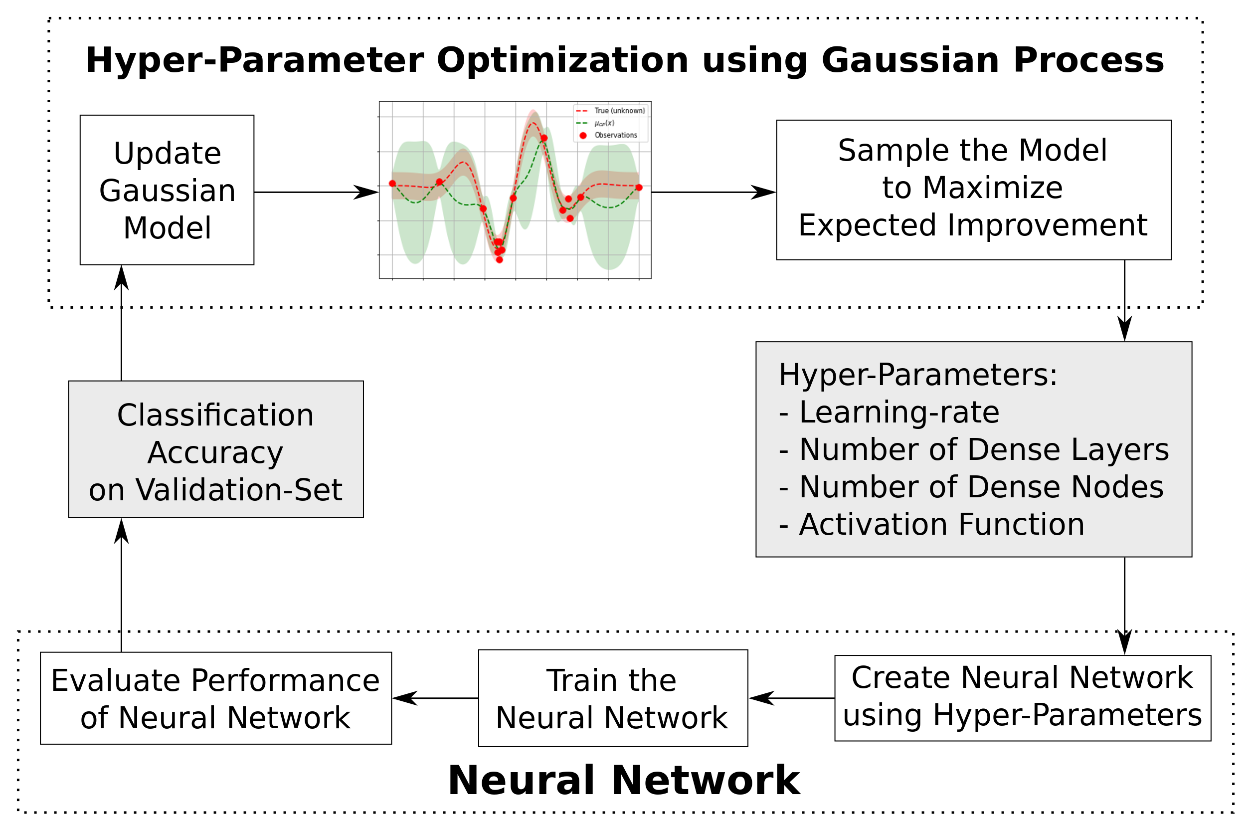
• This tutorial uses a clever method for finding good hyper-parameters known as Bayesian Optimization

Basic library from scikit-optimize

import skopt
from skopt import gp_minimize, forest_minimize
from skopt.space import Real, Categorical, Integer
from skopt.plots import plot_convergence
from skopt.plots import plot_objective, plot_evaluations
# from skopt.plots import plot_histogram, plot_objective_2D
from skopt.utils import use_named_args

Hyper parameter

dim_learning_rate = Real(low=1e-6, high=1e-2, prior='log-uniform',
                         name='learning_rate')


dim_num_dense_layers = Integer(low=1, high=5, name='num_dense_layers')

dim_num_dense_nodes = Integer(low=5, high=512, name='num_dense_nodes')

dim_activation = Categorical(categories=['relu', 'sigmoid'],
                             name='activation')

dimensions = [dim_learning_rate,
              dim_num_dense_layers,
              dim_num_dense_nodes,
              dim_activation]

Fitness Function

This is the function that creates and trains a neural network with the given hyper-parameters, and then evaluates its performance on the validation-set. The function then returns the so-called fitness value (aka. objective value), which is the negative classification accuracy on the validation-set. It is negative because skopt performs minimization instead of maximization.

Note the function decorator @use_named_args which wraps the fitness function so that it can be called with all the parameters as a single list, for example: fitness(x=[1e-4, 3, 256, 'relu']). This is the calling-style skopt uses internally.

@use_named_args(dimensions=dimensions)
def fitness(learning_rate, num_dense_layers,
            num_dense_nodes, activation):
    """
    Hyper-parameters:
    learning_rate:     Learning-rate for the optimizer.
    num_dense_layers:  Number of dense layers.
    num_dense_nodes:   Number of nodes in each dense layer.
    activation:        Activation function for all layers.
    """

    # Print the hyper-parameters.
    print('learning rate: {0:.1e}'.format(learning_rate))
    print('num_dense_layers:', num_dense_layers)
    print('num_dense_nodes:', num_dense_nodes)
    print('activation:', activation)
    print()
    
    # Create the neural network with these hyper-parameters.
    model = create_model(learning_rate=learning_rate,
                         num_dense_layers=num_dense_layers,
                         num_dense_nodes=num_dense_nodes,
                         activation=activation)

    # Dir-name for the TensorBoard log-files.
    log_dir = log_dir_name(learning_rate, num_dense_layers,
                           num_dense_nodes, activation)
    
    # Create a callback-function for Keras which will be
    # run after each epoch has ended during training.
    # This saves the log-files for TensorBoard.
    # Note that there are complications when histogram_freq=1.
    # It might give strange errors and it also does not properly
    # support Keras data-generators for the validation-set.
    callback_log = TensorBoard(
        log_dir=log_dir,
        histogram_freq=0,
        batch_size=32,
        write_graph=True,
        write_grads=False,
        write_images=False)
   
    # Use Keras to train the model.
    history = model.fit(x=data.train.images,
                        y=data.train.labels,
                        epochs=3,
                        batch_size=128,
                        validation_data=validation_data,
                        callbacks=[callback_log])

    # Get the classification accuracy on the validation-set
    # after the last training-epoch.
    accuracy = history.history['val_acc'][-1]

    # Print the classification accuracy.
    print()
    print("Accuracy: {0:.2%}".format(accuracy))
    print()

    # Save the model if it improves on the best-found performance.
    # We use the global keyword so we update the variable outside
    # of this function.
    global best_accuracy

    # If the classification accuracy of the saved model is improved ...
    if accuracy > best_accuracy:
        # Save the new model to harddisk.
        model.save(path_best_model)
        
        # Update the classification accuracy.
        best_accuracy = accuracy

    # Delete the Keras model with these hyper-parameters from memory.
    del model
    
    # Clear the Keras session, otherwise it will keep adding new
    # models to the same TensorFlow graph each time we create
    # a model with a different set of hyper-parameters.
    K.clear_session()
    
    # NOTE: Scikit-optimize does minimization so it tries to
    # find a set of hyper-parameters with the LOWEST fitness-value.
    # Because we are interested in the HIGHEST classification
    # accuracy, we need to negate this number so it can be minimized.
    return -accuracy

Run the Hyper-Parameter Optimization

search_result = gp_minimize(func=fitness,
                            dimensions=dimensions,
                            acq_func='EI', # Expected Improvement.
                            n_calls=40,
                            x0=default_parameters)

Result

plot_convergence(search_result)

search_result.x
space.point_to_dict(search_result.x)
search_result.fun
sorted(zip(search_result.func_vals, search_result.x_iters))
fig, ax = plot_histogram(result=search_result,
                         dimension_name='activation')

Bayesian Optimization Blog

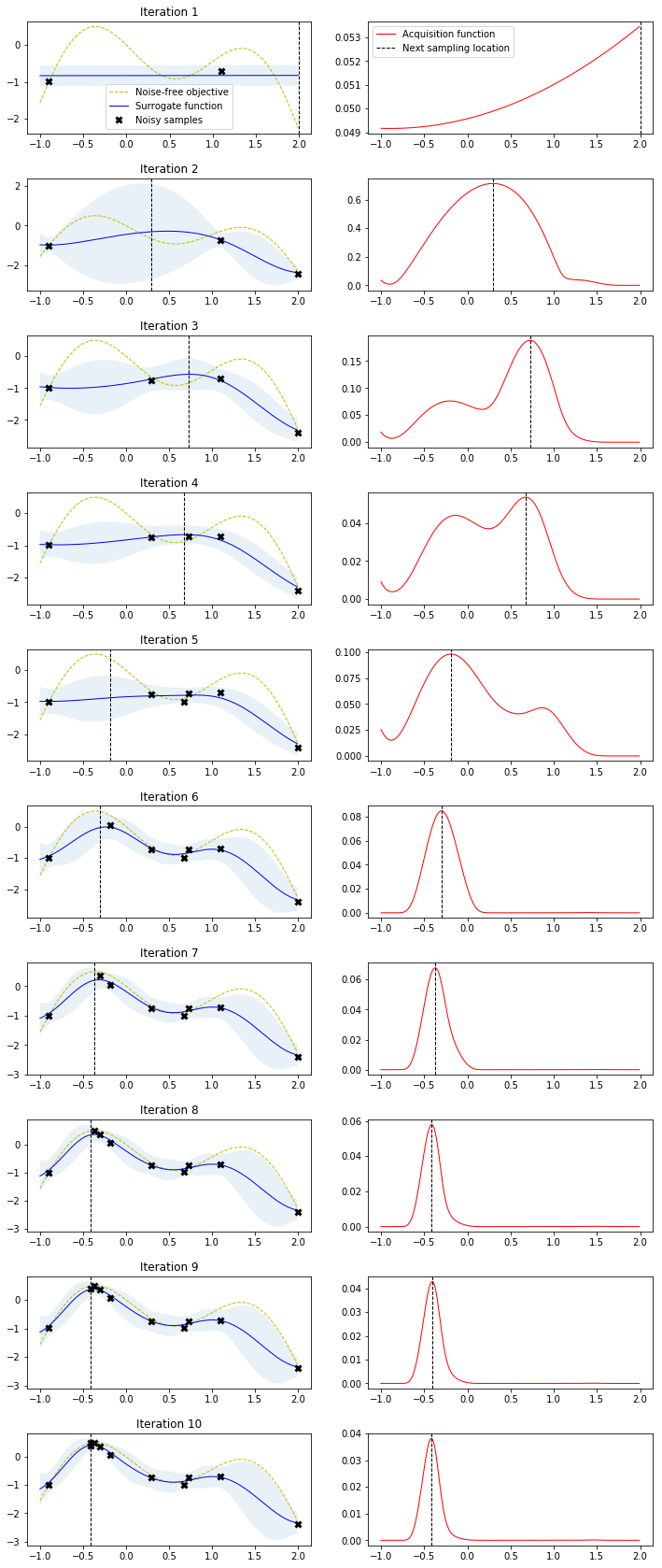
Scikit-optimize

from sklearn.base import clone
from skopt import gp_minimize
from skopt.learning import GaussianProcessRegressor
from skopt.learning.gaussian_process.kernels import ConstantKernel, Matern

# Use custom kernel and estimator to match previous example
m52 = ConstantKernel(1.0) * Matern(length_scale=1.0, nu=2.5)
gpr = GaussianProcessRegressor(kernel=m52, alpha=noise**2)

r = gp_minimize(lambda x: -f(np.array(x))[0], 
                bounds.tolist(),
                base_estimator=gpr,
                acq_func='EI',      # expected improvement
                xi=0.01,            # exploitation-exploration trade-off
                n_calls=10,         # number of iterations
                n_random_starts=0,  # initial samples are provided
                x0=X_init.tolist(), # initial samples
                y0=-Y_init.ravel())

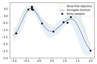
# Fit GP model to samples for plotting results
gpr.fit(r.x_iters, -r.func_vals)

# Plot the fitted model and the noisy samples
plot_approximation(gpr, X, Y, r.x_iters, -r.func_vals, show_legend=True)

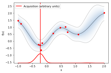
GPyOpt

import GPy
import GPyOpt

from GPyOpt.methods import BayesianOptimization

kernel = GPy.kern.Matern52(input_dim=1, variance=1.0, lengthscale=1.0)
bds = [{'name': 'X', 'type': 'continuous', 'domain': bounds.ravel()}]

optimizer = BayesianOptimization(f=f, 
                                 domain=bds,
                                 model_type='GP',
                                 kernel=kernel,
                                 acquisition_type ='EI',
                                 acquisition_jitter = 0.01,
                                 X=X_init,
                                 Y=-Y_init,
                                 noise_var = noise**2,
                                 exact_feval=False,
                                 normalize_Y=False,
                                 maximize=True)

optimizer.run_optimization(max_iter=10)
optimizer.plot_acquisition()