Behavioral Cloning in Autonomous Driving
Behaviroal Cloning in Autonomous Driving in Reinforcement Learning
Introduction
- Neural Network directly predicts the steering angles from the image of front camera
- The training data is only collected in track 1 by manually driving two laps and the neural network learns to drive the car on different tracks
Steps
- Use the simulator to collect data(front camera frames and steering angles) of good driving behavior on track 1
- Build a CNN in Keras that predicts steering angles from images
- Train and validate the model with a training and validation set on track 1
- Test that the model successfully drives around on both trained track 1 and unseen track 2
Codes
- model.py : containing the script to create and train the model
- drive.py : for driving the car in autonomous mode
- model.h5 containing a trained CNN
- environment-gpu.yml : environment file with GPU
- images folder contains the sample images
Dependencies
- OpenCV3,Python3.5,Keras,CUDA8.0
- GeForce GTX 980M, Intel Core i7
How to run the Code with pre-computed model
- using udacity simulator and drive.py file, the car can be driven autonomously around the track by following two steps:
- Launch Udacity simulator and enter AUTONOMOUS MODE
- Drive the car by executing
How to run the Code with your own model
- Launch the udacity simulator and enter TRAINING MODE
- Record your own manual driving sequences and save them as csv file
- Train your model with saved sequences
- Test your model in AUTONOMOUS MODE
Model Architecture
-
The model architecture
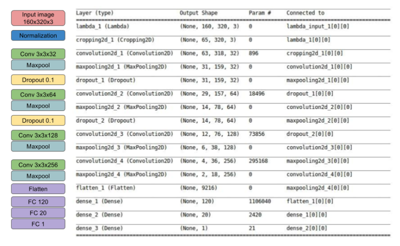
- CNN with 4 conv layers which have 3x3 filter sizes and depths vary between 32 and 256 and 3 fully connected layers
- The Model includes RELU layer to introduce nonlinearity
- And data is normalized in the model using a Keras lambda layer
- The model contains dropout layer in order to reduce overfitting
-
Training Strategy

- Training data from three cameras (left,center,right)
- record two laps on track 1 using center lane driving
- This is because we need to handle the issue of recovering from being off-center driving
- If we train the model to associate a given image from the center camera with a left turn, then we could also train the model to associate the left camera image with a somewhat softer left turn -And we could train the model to associate right camera image with an even harder left turn
- To estimate the steering angle of the left and right images, it uses a correction value of 0.2(in radians) in model.py
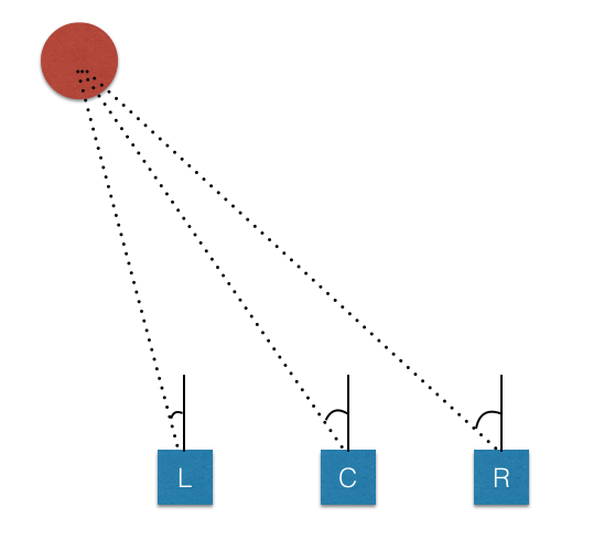
- It found this model doesn’t perform well in sharp turns
-
Data Augmentation
- Image Flipping : In track 1, most of the turns are left turns, so It flipped images and angles. As a result, the network would learn both left and right turns properly
- Brightness Changing : In order to learn a more general model,It randomly changes the image’s brightness in HSV space

-
Data Balancing
- Collected Data in not balanced, we can see the steering angle histogram as shown below and data balancing is a crucial step for network to have a good performance
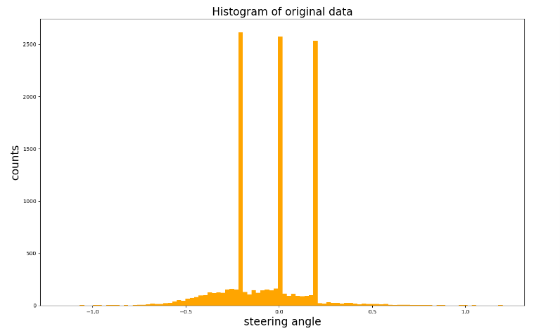
- In order to balance the data, we need to reduce the number of high bins, and it did it as in balance_data function in model.py
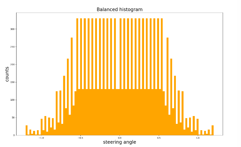
- Collected Data in not balanced, we can see the steering angle histogram as shown below and data balancing is a crucial step for network to have a good performance
-
Image Crop
- In the image, the up(sky) and bottom(front part of the car) are not very useful for training, and on the other hand, it might lead to overfitting
- this is done in GPU for efficiency

- When we process the left and right images, we add corrections(+0.2 and -0.2) for their steering angles because we know the ground-truth steering angle for the center camera
- The validation set helped determine if the model was over or under fitting
-
Model Design Approach
- This proposed model is derived from VGG and LeNet, which is more complex than LeNet but smaller than VGG
- This model had a low mean squared error on the training but a high mean squared error on the validation set -> This implied that the model was overfitting -> so add two dropout layer
Codes Analysis
# define the network model
model = network_model()
model.summary()
-
from keras.models import Sequential from keras.layers import Flatten, Dense, Lambda, Dropout from keras.layers.convolutional import Convolution2D, Cropping2D from keras.layers.pooling import MaxPooling2D def network_model(): model = Sequential() # normalization model.add(Lambda(lambda x: x / 127.5 - 1., input_shape=(160,320,3))) # Image Cropping model.add(Cropping2D(cropping=((70,25),(0,0)))) model.add(Convolution2D(32,3,3,activation='relu')) model.add(MaxPooling2D()) model.add(Dropout(0.1)) model.add(Convolution2D(64,3,3,activation='relu')) model.add(MaxPooling2D()) model.add(Dropout(0.1)) model.add(Convolution2D(128,3,3, activation='relu')) model.add(MaxPooling2D()) model.add(Convolution2D(256,3,3, activation='relu')) model.add(MaxPooling2D()) model.add(Flatten()) model.add(Dense(120)) model.add(Dense(20)) model.add(Dense(1)) return model 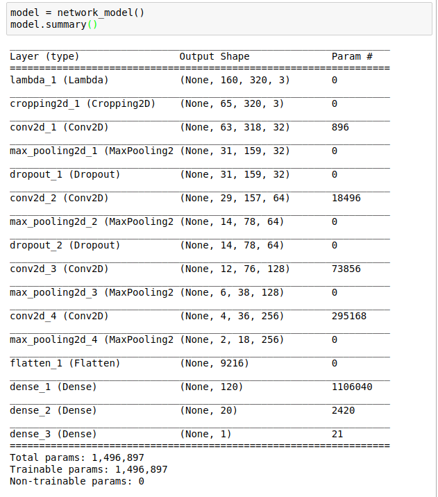
nbEpoch = 4
model.compile(loss='mse', optimizer='adam')
basePath = '/home/junsheng/Desktop/collect_tack1_alph/'
print('loading the data...')
samples = loadData(basePath)

# balance the data with smooth the histogram of steering angles
samples = balance_data(samples, visulization_flag=True)

# split data into training and validation
train_samples, validation_samples = train_test_split(samples, test_size=0.3)

# compile and train the model using the generator function
train_generator = generator(train_samples, train_flag=True, batch_size=32)
validation_generator = generator(validation_samples, train_flag=False, batch_size=32)

history = model.fit_generator(train_generator, samples_per_epoch=len(train_samples)*12, nb_epoch=nbEpoch,\
validation_data=validation_generator, nb_val_samples=len(validation_samples))
-
from sklearn.utils import shuffle from sklearn.model_selection import train_test_split def generator(samples, train_flag, batch_size=32): num_samples = len(samples) correction = 0.2 # correction angle used for the left and right # images while 1: # Loop forever so the generator never terminates shuffle(samples) for offset in range(0, num_samples, batch_size): batch_samples = samples[offset:offset+batch_size] images = [] angles = [] for line in batch_samples: angle = float(line[3]) c_imagePath = line[0].replace(" ", "") c_image = cv2.imread(c_imagePath) images.append(c_image) angles.append(angle) if train_flag: # only add left and right images for training data (not for validation) l_imagePath = line[1].replace(" ", "") r_imagePath = line[2].replace(" ", "") l_image = cv2.imread(l_imagePath) r_image = cv2.imread(r_imagePath) images.append(l_image) angles.append(angle + correction) images.append(r_image) angles.append(angle - correction) # flip image and change the brightness, for each input image, returns other 3 augmented images augmented_images, augmented_angles = data_augmentation(images, angles) X_train = np.array(augmented_images) y_train = np.array(augmented_angles) yield shuffle(X_train, y_train) -
def balance_data(samples, visulization_flag ,N=60, K=1, bins=100): ... """ Crop the top part of the steering angle histogram, by removing some images belong to those steering angels :param images: images arrays :param angles: angles arrays which :param n: The values of the histogram bins :param bins: The edges of the bins. Length nbins + 1 :param K: maximum number of max bins to be cropped :param N: the max number of the images which will be used for the bin :return: images, angle """ n, bins, patches = plt.hist(angles, bins=bins, color= 'orange', linewidth=0.1) angles = np.array(angles) n = np.array(n) idx = n.argsort()[-K:][::-1] # find the largest K bins del_ind = [] # collect the index which will be removed from the data for i in range(K): if n[idx[i]] > N: ind = np.where((bins[idx[i]]<=angles) & (angles<bins[idx[i]+1])) ind = np.ravel(ind) np.random.shuffle(ind) del_ind.extend(ind[:len(ind)-N]) # angles = np.delete(angles,del_ind) balanced_samples = [v for i, v in enumerate(samples) if i not in del_ind] balanced_angles = np.delete(angles,del_ind) ... - plt.hist and numpy array example
  mu, sigma = 100, 15
  bins = 10
  angles = mu+sigma*np.random.randn(1000)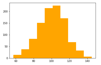
  n, bins, patches = plt.hist(angles, bins=bins, color= 'orange', linewidth=0.1)
  angles = np.array(angles)
  n = np.array(n)
  # print(len(angles))
  # >> 1000
  # print(max(angles),min(angles))
  # >> 144.74294725445378 57.47568825996446
  # print (sum(n))
  # >> 1000.0
  # print(n) # y-axis
  # >> [ 14.  38.  82. 151. 214. 225. 170.  68.  32.   6.]
  # print(bins) # x-axis
  # >> [ 57.47568826  66.20241416  74.92914006  83.65586596  92.38259186
  #      101.10931776 109.83604366 118.56276956 127.28949546 136.01622136
  #      144.74294725]

  idx = n.argsort()[-K:][::-1]    # find the largest K bins
  # idx -> array([5]) in this example
  # idx = n.argsort()
  # >> array([9, 0, 8, 1, 7, 2, 3, 6, 4, 5])
  # K = 1
  # idx = n.argsort()[-K:][::-1]
  # idx
  # >> array([5])
  # idx[0]
  # >> 5
  # n[5]
  # >> 225
  del_ind = [] # collect the index which will be removed from the data
  for i in range(K):
      if n[idx[i]] > N:
          ind = np.where((bins[idx[i]]<=angles) & (angles<bins[idx[i]+1]))
          ind = np.ravel(ind)
          np.random.shuffle(ind)
          del_ind.extend(ind[:len(ind)-N])

  # n[idx[0]] -> 225 : the most frequency number
  # np.where((bins[idx[i]]<=angles) & (angles<bins[idx[i]+1])) returns
  # indexes of angles between bins[idx[0]] and bins[idx[0]+1]
  # bins[idx[0]],bins[idx[0]+1] # in angles
  # >> (101.10931775720913, 109.83604365665806)
  # len(ind[0])
  # >> 225
  # angles[ind[0][0]] , angles[ind[0][-1]]
  # >> (102.55220459373017, 109.5420984773099)
matplotlib.plt.hist np.ravel keras_fit_generator keras fit_generator