Hvass forecast stock returns
Data Sources
- Price data from Yahoo Finance.
- Financial data for individual stocks collected manually by the author from the 10-K Forms filed with the U.S. SEC.
- Newer S&P 500 data from the S&P Earnings & Estimates Report and older data from the research staff at S&P and Compustat (some older data is approximated by their research staff).
- U.S. Government Bond yield for 1-year constant maturity. From the U.S. Federal Reserve.
- The inflation index is: All Items Consumer Price Index for All Urban Consumers (CPI-U), U.S. City Average. From the US Department of Labor, Bureau of Labor Statistics.
Forecasting Long-Term Stock Returns
Introduction
- For shorter investment periods, the P/Sales ratio is found to be a weak predictor for the stock’s return, but for longer periods of 10 years, the P/Sales ratio is a strong predictor for the return of the S&P 500 and some indivisual stocks
- This is a very important discovery and it has implications for many areas of both theoretical and applied finance
- It means that U.S stock market as a whole is not efficient and does not follow random walk in the long-term
- It is possible to estimate the future long term return of the stock market and some indivisual stocks from a single indicator variable
- The core idea comes from the author’s research book from the year 2015: Strategies for Investing in the S&P 500
- Hidden deep inside that book in Section 13.1.4 on page 84, the following formula is found for predicting the 10-year annualized return of the S&P 500
- In this work we will primarily use the P/Sales ratio as the predictor variable instead, because the historical P/Sales ratio may be easier to obtain for some companies, and because the P/Book ratio is more sensitive to changes in capitalization structure for individual companies
Python Imports
%matplotlib inline

import matplotlib.pyplot as plt
from matplotlib.ticker import FuncFormmater
import pandas as pd
import numpy as np
import os

from curve_fit import CurveFitLinear,CurveFitReciprocal
from data_keys import *
from data import load_index_data,load_stock_data,load_usa_cpi
from returns import annualized_returns, prepare_ann_returns
Load Data
# Define the ticker-names for the stocks we consider.
ticker_SP500 = "S&P 500"
ticker_JNJ = "JNJ"
ticker_K = "K"
ticker_PG = "PG"
ticker_WMT = "WMT"

# Load the financial data for the stocks.
df_SP500 = load_index_data(ticker=ticker_SP500)
df_JNJ = load_stock_data(ticker=ticker_JNJ)
df_K = load_stock_data(ticker=ticker_K)
df_PG = load_stock_data(ticker=ticker_PG)
df_WMT = load_stock_data(ticker=ticker_WMT)

# Load the US CPI inflation index.
cpi = load_usa_cpi()
Plotting Functions
def normalize(x):
    y = (x - x.min())
    y /= y.max()
    return y

SALES_PER_SHARE = "Sales Per Share"
BOOK_VALUE_PER_SHARE = "Book-Value Per Share"
TOTAL_RETURN = 'Total Return'

def plot_total_return_sales_book_value(df,ticker):
    # Copy the relevant data
    df2 = df[[SALES_PER_SHARE,
              BOOK_VALUE_PER_SHARE,
              TOTAL_RETURN]].copy()
    # Drop all rows with NA
    df2.dropna(axis=0,how='any',inplace=True)

    # Normalize the data to be between 0 and 1
    df2[TOTAL_RETURN] = normalize(df2[TOTAL_RETURN])
    df2[SALES_PER_SHARE] = normalize(df2[SALES_PER_SHARE])
    df2[BOOK_VALUE_PER_SHARE] = normalize(df2[BOOK_VALUE_PER_SHARE])

    df2.plot(title=ticker)
def plot_scatter_fit(ax,years,ticker,x,y,x_name):
ax,scatter(x,y)
title1 = "[{0}] {1}-Year Ann. Return".format(ticker,years)
x_min = np.min(x)
x_max = np.max(x)
curve_fit_linear = CurveFitLinear(x=x, y=y)
x_range = np.array([x_min, x_max])
y_pred = curve_fit_linear.predict(x=x_range)
ax.plot(x_range, y_pred, color='black')
# Title with these curve-fit parameters.
title2 = "black = {0:.1%} x " + x_name + " + {1:.1%}"
title2 = title2.format(*curve_fit_linear.params)
...
formatter = FuncFormatter(lambda y, _: '{:.0%}'.format(y))
ax.yaxis.set_major_formatter(formatter)
def plot_ann_returns(ticker,df,key=PSALES):
fig,axes = plt.subplot(5,2,figsize=(10,20))
fig.subplots_adjust(hspace=0.6,wspace=0.15)
for i,ax in enumerate(axes.flat):
years = i + 1
x, y = prepare_ann_returns(df=df,years=years,key=key)
plot_scatter_fit(ax=ax,years=years,x_name=key,ticker=ticker,x=x,y=y)
...
plt.show()
def plot_ann_returns_adjusted(ticker,df,years,subtract,key=PSALES):
fig = plt.figure(figsize=(10,10))
ax = fig.add_subplot(211)
x,y = prepare_ann_returns(df=df,years=years,
subtract=subtract, key=key)
plot_scatter_fit(..)
plt.show()
def plot_total_return(df,ticker,start_date=None):
tot_ret = df[TOTAL_RETURN][start_date:].dropna()
tot_ret /= tot_ret[0]
tot_ret.plot(title=ticker+" - Total Return",grid=True)
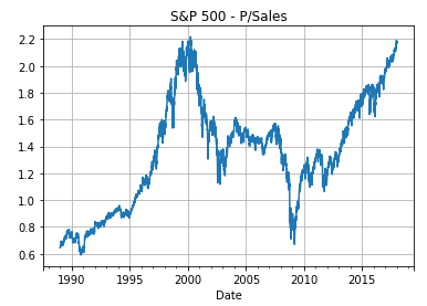
def plot_psales(df,ticker,start_date=None):
psales = df[PSALES][start_date:].dropna()
psales.plot(title=ticker + " - P/Sales", grid=True)
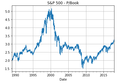
def plot_pbook(df, ticker, start_date=None):
pbook = df[PBOOK][start_date:].dropna()
pbook.plot(title=ticker + " - P/Book", grid=True)
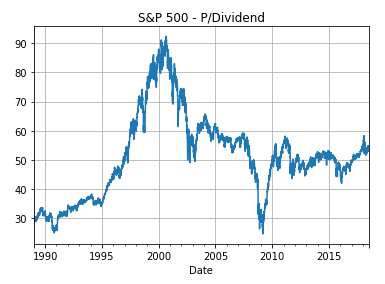
def plot_pdividend(df, ticker, start_date=None):
pdividend = df[PDIVIDEND][start_date:].dropna()
pdividend.plot(title=ticker + " - P/Dividend", grid=True)
S&P 500
- The S&P 500 covers about 80% of the whole US stock market in terms of size so it is useful as a gauge for the entire US stock market
- We consider the Total Return of the S&P 500 which is what you would get from investing in the S&P 500 and re investing all dividends back into the S&P 500
start_date = df_SP500[PSALES].dropna().index[0]
plot_total_return(df=df_SP500, ticker=ticker_SP500,
                  start_date=start_date)

df_SP500[-10:]
>>
    Total Return    Share-price     Dividend    Sales Per Share     P/Sales     Book-Value Per Share    P/Book  Dividend TTM    Dividend Yield  P/Dividend
Date
2018-06-27  1513.453527     2699.629883     NaN     NaN     NaN     NaN     NaN     50.968478   0.018880    52.966657
2018-06-28  1522.804688     2716.310059     NaN     NaN     NaN     NaN     NaN     50.979239   0.018768    53.282672
2018-06-29  1531.303646     2718.370117     13.1    NaN     NaN     NaN     NaN     50.990000   0.01
- The P/Sales ratio is defined as the price per share dividied by the salesper share for the past 12 months
plot_psales(df=df_SP500, ticker=ticker_SP500, start_date=start_date)
plot_pbook(df=df_SP500, ticker=ticker_SP500, start_date=start_date)
plot_pdividend(df=df_SP500, ticker=ticker_SP500, start_date=start_date)
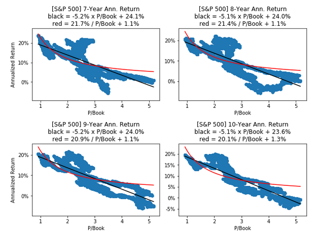
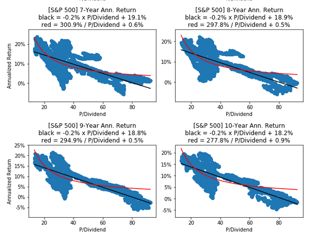
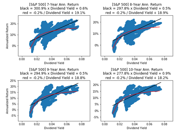
S&P 500 P/Sales vs Annualized Returns
- The following scatter-plots show the P/Sales ratio versus the Annualized Returns of the S&P 500 for periods from 1 to 10 years.
- For example, the last plot is for 10-year investment periods
- we calculate the Annualized Return from that, and then we put a blue dot in the scatter-plot for that date’s P/Sales ratio and the Annualized Return we just calculated
plot_ann_returns(ticker=ticker_SP500, df=df_SP500, key=PSALES)
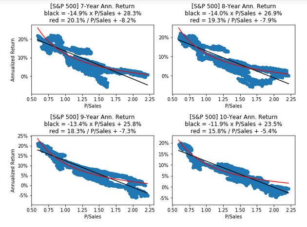
- The first plot shows 1-year investment periods and has a large “blob” of blue dots with poorly fitted return-curves. This means the P/Sales ratio is a weak predictor for the 1-year returns of the S&P 500
- This makes sense because in the short-term the P/Sales ratio only changes because of the share-price as the sales-per-share is almost constant in the short-term. And it seems highly unlikely that we can predict future returns from the share-price alone
- The last plot shows 10-year investment periods where the curves fit the blue dots quite well, so the P/Sales ratio is a strong predictor for 10-year returns of the S&P 500
- In the following, we will sometimes refer to these fitted curves as “Return Curves”
plot_ann_returns(ticker=ticker_SP500, df=df_SP500, key=PBOOK)
plot_ann_returns(ticker=ticker_SP500, df=df_SP500, key=PDIVIDEND)
plot_ann_returns(ticker=ticker_SP500, df=df_SP500, key=DIVIDEND_YIELD)
S&P 500 - Forecasting Next 10-Year Return using P/Sales
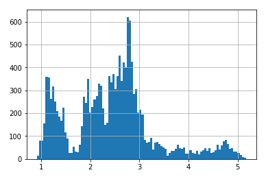
- Towards the end of 2017, the P/Sales ratio was about 2.2 for the S&P 500
- We can forecast the 10-year annualized returns using the fitted “return curves” and formulas from the plots above
- If you purchased the S&P 500 in December 2017 and will keep the investment until the end of 2027 while reinvesting all dividends during those 10 years (all taxes are ignored), then the formula forecasts this return
- This means that you would lose an estimated -2.7% per year on your investment in the S&P 500 between December 2017 and December 2027, according to this formula
- Let us plot a histogram of the historical P/Sales data where we can also see that the P/Sales ratio of 2.2 is at the very top, so the S&P 500 was indeed priced historically high in December 2017 according to this metric
df_SP500[PSALES].hist(bins=100, grid=True)
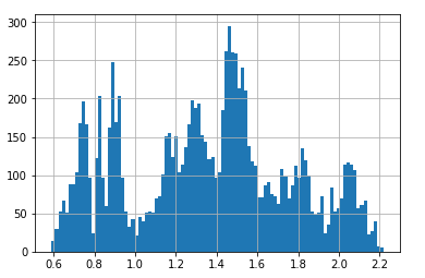
S&P 500 - Forecasting Next 10-Year Return using P/Book
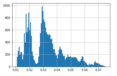
We can also use the formula with the P/Book ratio instead. Towards the end of 2017 the P/Book ratio was about 3.2 for the S&P 500. The formula then gives the forecasted return:
\[Annualized\ Return = -5.1\% \cdot P/Book + 23.6\% = -5.1\% \cdot 3.2 + 23.5\% \simeq 7.2\%\]This is much different than the forecasted annual loss of -2.7% when using the formula with the P/Sales ratio instead. It is unclear why the two formulas give such different forecasts. Maybe it is related to higher profit-margins and debt-to-equity ratios, but a deeper investigation of the financial data would be needed to uncover a plausible reason.
We can also show a histogram of the historical P/Book ratios for the S&P 500, where the P/Book value of 3.2 can be seen to be at the start of the distributions’ higher end.
S&P 500 - Forecasting Next 10-Year Return using Dividend Yield
We can also use the formula with the dividend yield instead. Towards the end of 2017 the dividend yield was about 1.8% for the S&P 500. The formula then gives the forecasted return:
\[Annualized\ Return = -0.2\% / Dividend\ Yield + 17.6\% = -0.2\% / 1.8\% + 17.6\% \simeq 6.5\%\]This is fairly close to the forecasted return of 7.2% when using the P/Book ratio above.
We can also show a histogram of the historical dividend yields for the S&P 500, where a dividend yield of 1.8% is at the lower end of the distribution, corresponding to a historically high valuation for the shares because the dividend yield is the inverse of the P/Dividend ratio.
Theoretical Explanation
We have found a strong predictive relationship between the P/Sales or P/Book ratios and the long-term return of the S&P 500 and some individual stocks. Let us now discuss what may be the cause of this relationship and whether it can be expected to continue in the future, so the formulas above can be used to forecast the future returns of the S&P 500 and those individual stocks.
Random Walk?
For several decades, most finance professors have believed that stock-prices fluctuate completely randomly and cannot be predicted by any means. This may be partially true in the short-term, but it is not true in the long-term because it completely ignores the fact that shares represent part ownership in the underlying businesses, which have real assets, real sales, and real profits that do not fluctuate completely randomly.
The world’s all-time best long-term investor is Warren Buffett who learnt investment finance from a man named Ben Graham who used to say that in the short-term the stock-market is a voting machine, but in the long-term the stock-market is a weighing machine. By this he meant that the stock-market does seem to fluctuate randomly in the short-term, but in the long-term the economics of the underlying businesses will dominate the returns of stocks.
When we consider the S&P 500 stock-market index it is really a gauge of all U.S. businesses because the index covers about 80% of the publicly traded companies in terms of size. So we would expect the return of the S&P 500 to roughly follow the growth in the U.S. economy over longer periods of time. But the stock-prices do fluctuate randomly every day, so how does that affect the long-term returns?
Intrinsic Value
We can better understand this if we consider the intrinsic value (or true underlying value) of a stock to be different from the current share-price. For example, if the underlying business of a stock grows 9% per year for 10 years, then the intrinsic value after 10 years has become:
\[Intrinsic\ Value_{10\ Years} = Intrinsic\ Value_{Today} \cdot 1.09 ^ {10}\]If we could buy and sell a company’s stock for a price equal to the intrinsic value - and we ignore dividends for now - then the investor’s return would simply be 9% compounded for 10 years:
\[Return = \frac{Intrinsic\ Value_{10\ Years}}{Intrinsic\ Value_{Today}} = 1.09 ^ {10}\]But the problem is that nobody knows what the intrinsic value of a business is, because it depends on future earnings which are impossible to know in advance. So there is a lot of guessing when the stock-market tries to establish a fair price for a stock.
Furthermore, because stocks can be bought and sold almost instantly, many market participants are not long-term investors but short-term speculators. This means the share-price may fluctuate significantly during a day even though the intrinsic value of the underlying business has not changed at all.
Intrinsic Value vs. Share-Price
Instead of considering the share-price to be completely random, we should instead consider it to be a random variable that fluctuates around the intrinsic value of the underlying business. We can write it like this for some random number drawn from an unknown distribution:
\[Share\ Price = Intrinsic\ Value \cdot Random\]We might call this random number for the mispricing factor, as it causes the shares to be mispriced for all random values except 1.
Now the return we get on the investment is affected by the growth in the intrinsic value as well as the two random variables for the buying and selling prices of the stock:
\[Return_{10\ Years} = \frac{Share\ Price_{10\ Years}}{Share\ Price_{Today}} = \frac{Intrinsic\ Value_{10\ Years} \cdot Random_{10\ Years}}{Intrinsic\ Value_{Today} \cdot Random_{Today}}\]If we still assume the intrinsic value grows 9% per year then we get:
\[Return_{10\ Years} = 1.09 ^ {10} \cdot \frac{Random_{10\ Years}}{Random_{Today}}\]Total Return vs. Share-Price
In the formulas above we ignored dividends that would be paid out during the investment period of 10 years and reinvested immediately into the same stock. We assume there are no taxes when reinvesting dividends and we call the result for the Total Return of the stock.
We may consider the Total Return by including a share-count in the formula:
\[Return_{10\ Years} = \frac{Shares_{10\ Years} \cdot Share\ Price_{10\ Years}}{Shares_{Today} \cdot Share\ Price_{Today}} \\ = \frac{Shares_{10\ Years} \cdot Intrinsic\ Value_{10\ Years} \cdot Random_{10\ Years}}{Shares_{Today} \cdot Intrinsic\ Value_{Today} \cdot Random_{Today}}\]where the number of shares starts at 1 and increases slightly whenever a dividend is paid out and reinvested into the same stock, according to this formula:
\[Shares_t = Shares_{t-1} \cdot (1 + \frac{Dividend_t}{Share\ Price_t})\]Notice that when calculating the return, the growth in share-count could simply be replaced by an increased growth in the intrinsic value and the result would be identical. In the examples and simulations further below, we will therefore combine these into a single growth-rate to keep the notation simple.
Annualized Return
We can then calculate the annualized return for investment periods of $N$ years as follows:
\[Annualized\ Return = (\frac{Shares_{N\ Years} \cdot Share\ Price_{N\ Years}}{Shares_{Today} \cdot Share\ Price_{Today}}) ^ {1/N} - 1 \\ = (\frac{Shares_{N\ Years}}{Shares_{Today}}) ^ {1/N} \cdot (\frac{Intrinsic\ Value_{N\ Years}}{Intrinsic\ Value_{Today}}) ^ {1/N} \cdot (\frac{Random_{N\ Years}}{Random_{Today}}) ^ {1/N} - 1\]This makes it clear that the annualized return depends on three things: The annualized return in the intrinsic value, the annualized return in the number of shares from reinvestment of dividends, and the annualized return from the mispricing of the stock at the time of buying and selling.
The random mispricing factors are assumed to be limited e.g. between 0.5 and 2.0 so that the share-price fluctuates around the intrinsic value per-share. This means the annualized return on the mispricing factor goes towards 1.0 as the number of years $N$ increases, so in the long-term the annualized return on the stock is dominated by the growth in the intrinsic value and the share-count from reinvestment of dividends:
\[\lim_{N \rightarrow \infty} Annualized\ Return = (\frac{Shares_{N\ Years}}{Shares_{Today}}) ^ {1/N} \cdot (\frac{Intrinsic\ Value_{N\ Years}}{Intrinsic\ Value_{Today}}) ^ {1/N} - 1\]Examples
Let us consider a few examples of random factors for the buying and selling prices.
First consider the case where the stock is priced exactly at the intrinsic value when it is sold so that $Random_{10\ Years} = 1$, but there is a 20% under-pricing at the time of purchase so that $Random_{Today} = 0.8$. We assume the intrinsic value and share-count from reinvestment of dividends grows at a combined 9% every year. Using the formula above, the annualized return on the stock is then:
\[Annualized\ Return = (\frac{Shares_{N\ Years} \cdot Intrinsic\ Value_{N\ Years}}{Shares_{Today} \cdot Intrinsic\ Value_{Today}}) ^ {1/N} \cdot (\frac{Random_{10\ Years}}{Random_{Today}}) ^ {1/10} - 1 \\ = 1.09 \cdot (\frac{1}{0.8}) ^ {1/10} - 1 \simeq 11.5\% \\\]Now consider the opposite case where $Random_{10\ Years} = 1$ but there is now a 20% over-pricing at the time of purchase so that $Random_{Today} = 1.2$. We get:
\[Annualized\ Return = 1.09 \cdot (\frac{Random_{10\ Years}}{Random_{Today}}) ^ {1/10} - 1 \\ = 1.09 \cdot (\frac{1}{1.2}) ^ {1/10} - 1 \simeq 7.0\% \\\]Similarly we can assume the buying stock-price is equal to the intrinsic value so $Random_{Today} = 1$ but now the selling price is 20% below the intrinsic value of the stock so $Random_{10\ Years} = 0.8$. We then get the annualized return:
\[Annualized\ Return = 1.09 \cdot (\frac{Random_{10\ Years}}{Random_{Today}}) ^ {1/10} - 1 \\ = 1.09 \cdot (\frac{0.8}{1}) ^ {1/10} - 1 \simeq 6.6\% \\\]Or we can assume that $Random_{Today} = 1$ but the stock is 20% over-priced when sold so that $Random_{10\ Years} = 1.2$. This gives us:
\[Annualized\ Return = 1.09 \cdot (\frac{Random_{10\ Years}}{Random_{Today}}) ^ {1/10} - 1 \\ = 1.09 \cdot (\frac{1.2}{1}) ^ {1/10} - 1 \simeq 11.0\% \\\]So we see that the annualized return also fluctuates randomly around the combined growth-rate for the intrinsic value and share-count, when the share-price fluctuates randomly around the intrinsic value.
You can try this formula with different choices of intrinsic growth-rate, investment years and random numbers for the buying and selling prices.
Conclusion
We have shown that there is a strong empirical relationship between the P/Sales ratio and the long-term returns of the S&P 500 stock-market index as well as some individual stocks. For short-term investment periods of only a few years or less, the P/Sales ratio was found to be a weak predictor for the stock returns.
We have also provided a simulation model along with an explanation for the observed relationship between the P/Sales ratio and future stock returns. The model basically split the share-price into two components: The intrinsic value and a random factor. This caused the share-price to fluctuate randomly around the intrinsic value, which was assumed to have more stable growth. It was then demonstrated using simulations, that the stock return was dominated in the long-term by the growth in the intrinsic value, but it was dominated in the short-term by the random fluctuations in share-price. Furthermore, the simulation model showed that it was possible to estimate the long-term future stock return based on the degree of mispricing at the time the stock was purchased, similar to what we observed for the S&P 500 index and some individual stocks.
In the real world, the mispricing of a stock cannot be measured in absolute terms, but it can be gauged in relative terms e.g. by using the P/Sales ratio, provided the company’s future sales-growth and net profit margin is similar to its past. This allows us to fit a curve on a scatter-plot of the historical P/Sales ratio versus the annualized returns e.g. for all 10-year investment periods, and use the fitted formula to forecast the future returns.
However, before using these formulas to forecast the future returns of a stock, you must convince yourself that the future of the company is probably going to be somewhat similar to its past in terms of sales-growth and profit-margin. This is very much a qualitative assessment of the company’s future.
If you think the company or perhaps the whole stock-market will experience unprecedented sales-growth or decline in the future, then you can still use the forecasts as base-estimates and then make appropriate adjustments.
For example, at the depths of a market-crash the formula might forecast a 20% annualized return for a 10-year investment in the S&P 500. So you can ask yourself if it seems justified that the U.S. economy has suffered so great damage that the future revenue of U.S. companies will be less than half of what they were just a few years ago. Unless USA has suffered a nuclear attack or a natural disaster on an epic scale, that seems highly unlikely.
Conversely, during stock-market euphoria with very high stock-prices, the formula might predict an annualized loss of -5% for a 10-year investment in the S&P 500. So now you can ask yourself if the U.S. economy is likely going to grow substantially more than it has done in the past, or whether it means that the stock-market is currently overpriced.
Research Ideas
You are strongly encouraged to do more research on this topic. If you make any new discoveries then please let me know your results.
To my knowledge, there are no academic studies of predicting the long-term returns of stocks and stock-markets as we have done here. This work has presented the basic idea and methodology, but a lot more research can be done on this subject and it may impact many areas of both theoretical and applied finance.
Here are some ideas you could start researching:
- Use proper statistical methods to measure the strength of the predictive relationship.
- Use other financial ratios as the predictor variable, for example the P/Dividend or P/Earnings ratio (maybe use a rolling 5-year average of earnings). Does it make sense to use those predictor variables? What are the pros and cons of each predictor variable?
- Can you use other economic indicators as predictor variables, such as the unemployment rates, interest rates, currency exchange rates, etc. Does that even make sense? If you find a predictive relationship is it actually causal or is it merely a correlation? How would you test this?
- Can you use industry-specific data as predictor variables for individual companies or sector-indices?
- Use multiple predictor variables together. Does it improve the accuracy of the prediction?
- Find some companies where you have data for at least 20-30 years, but where there is no predictive relationship between P/Sales and 10-year returns. Examine the history of the company and explain why that might be. Maybe the company has fundamentally changed its business and that explains it?
- Find some really old companies where the data for the share-price and P/Sales is available for many decades.
- Try and use other stock-market indices for individual sectors or other countries. You probably need data for at least 20-30 years which may be difficult or impossible to obtain. Perhaps you can build an index yourself?
- How would you use the predictive formulas in portfolio allocation?
- How would you use the predictive formulas for calculating discount rates used in valuation?
- Make simulations with random growth for the intrinsic value. Does it change the results substantially, or do you still observe the same kind of relationship between the
random_buyvariable and the annualized returns? - Make simulations with different growth-rates in intrinsic value, then fit the return curves and see how well they predict the future returns when the growth is different. Can they still be used as a rough estimate for the future returns, or are they completely inaccurate?
- Make simulations using a small subset of real-world data e.g. for the S&P 500 index and see how well the fitted curves predict actual returns on the full data-period. Can this be used to make predictions for stock-indices where you only have data for a few years? Would this work for individual companies or why not?