Simple Reinforcement Learning with Tensorflow Part 7: Action-Selection Strategies for Exploration

Introduction

• It will go over a few of the commonly used approaches to exploration which focus on action-selection and show their strengths and weakness

Why Explore?

• In order for an angent to learn how to deal optimally with all possible states,it must be exposed to as many as those states as possible
• Unlike supervised learning, the agent in RL has access to the environment through its own actions
• An Agent needs the right experiences to learn a good policy, but it also needs a good policy to obtain those experience
• exploration and exploitation tradeoff

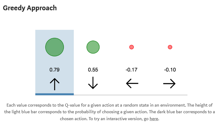
Greedy Approach

Explanation

• All RL seeks to maximize reward over time
• A greedy method
  • Taking the action which the agent estimates to be the best at the current moment is exploitation
  • This approach cab be thought of as providing little to no exploratory potential

Shortcomings

• The problem is it almost arrives at a suboptimal solution
• Imagine a simple two-armed bandit problem
  • If we suppose one arm gives a reward of 1 and the other arm gives a reward of 2, then if the agent’s parameters are such that it chooses the former arm first, then regardless of how complex a neural network we utilize, under a greedy approach it will never learn that the latter action is more optimal

Implementation

#Use this for action selection.
#Q_out referrs to activation from final layer of Q-Network.
Q_values = sess.run(Q_out, feed_dict={inputs:[state]})
action = np.argmax(Q_values)

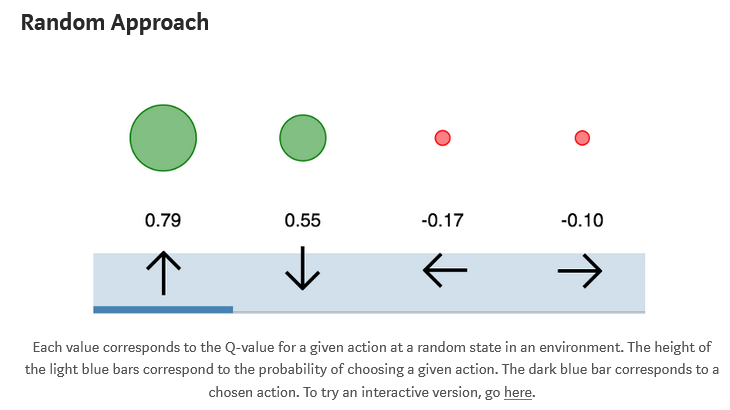
Random Approach

Explanation

• It is to simply always take a random action

Shortcomings

• It can be useful as an initial means of sampling from the state space in order to fill an experience buffer when using DQN

Implementation

#Assuming we are using OpenAI gym environment.
action = env.action_space.sample()

#Otherwise:
#total_actions = ??
action = np.random.randint(0,total_actions)

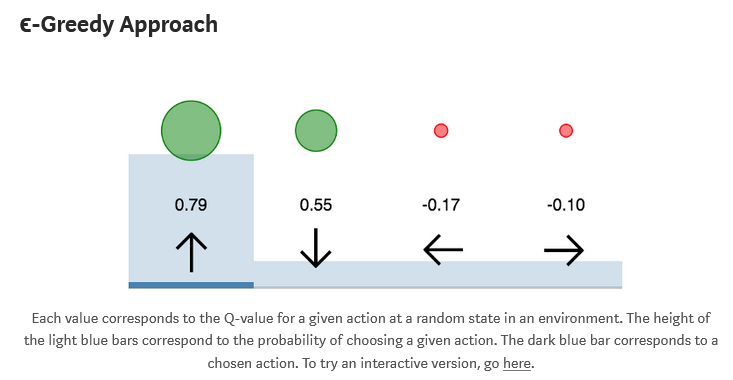
e-greedy Approach

Explanation

• A simple combination of the greedy and random approaches yields one of the most used exploration strategies
• The agent chooses what it believes to be the optimal action most of the time,but occasionally acts randomly
• The epsion parameter determines the probability of taking a random action
• The most defacto technique in RL

Adjusting during training

• At the start of the training process the e value is initialized to a large probability, to encourage exploration
• The e value is then annealed down to the small constant (0.1), as the agent is assumed to learn most of what it needs the environment

Shortcomings

• This method is far from the optimal,it takes into account only whether actions are most rewarding or not

Implementation

e = 0.1
if np.random.rand(1) < e:
    action = env.action_space.sample()
else:
    Q_dist = sess.run(Q_out,feed_dict={inputs:[state]})
action = np.argmax(Q_dist)

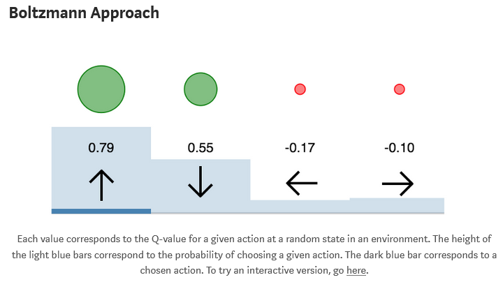
Boltzmann Approach

Explanation

• It would ideally like to exploit all the information present in the estimated Q values
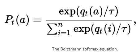
• Instead of always taking the optimal action or taking random action, this approach involves choosing an action with weighted probabilities
• To accomplish this we use a softmax over the networks estimates to be optimal is to be choosen
• The biggest advantage over e-greedy is that value of the other actions can also be taken into consideration
• If there are 4 actions available, in e-greedy the 3 actions estimated to be non-optimal are all considered equally, but in Boltzmann exploration they are weighted by their relative value
• This way the agent can ignore actions which it estimates to be largely sub-optimal and give more attention to potentially promising

Adjusting during training

• we utilize an additional temerature parameter which is annealed over time
• This parameter controls the spread of the softmax distribution
• such that all actions are considered equally at the start of training, and actions are sparsely distributed by the end of training

Shortcomings

• The softmax over network outputs provides a measure of the agent’s confidence in each action
• Instead what the agent is estimating is a measure of how optimal the agent thinks the action is, not how certain it is about that optimality

Implementation

#Add this to network to compute Boltzmann probabilities.
Temp = tf.placeholder(shape=None,dtype=tf.float32)
Q_dist = slim.softmax(Q_out/Temp)

#Use this for action selection.
t = 0.5
Q_probs = sess.run(Q_dist,feed_dict={inputs:[state],Temp:t})
action_value = np.random.choice(Q_probs[0],p=Q_probs[0])
action = np.argmax(Q_probs[0] == action_value)

Bayesian Approaches (w/Dropout)

Explanation

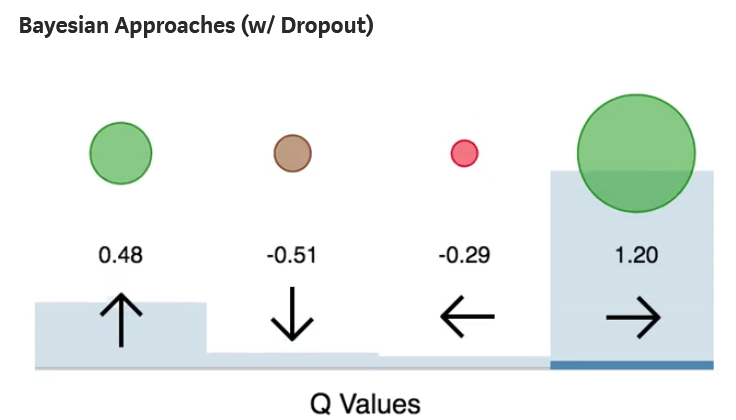
• What if an agent exploit its own uncertainty about its actions?
  • This is exactly the ability that a class of neural network models referred to as Bayesian Neural Network provide
• BNNs act probabilistically
  • This means that instead of having a single set of fixed weights, a BNNs maintains a probability distribution over possible weights
• In a RL, the distribution over weight values allows us to obtain distributions over actions as well
• The variance of this distribution provides us an estimate of the agent’s uncertainty about each action

Shortcomings

• In order to get true uncertainty estimates, multiple samples are required
• In order to reduce the noise in the estimate, the dropout keep probability is simply annealed over time from 0.1 to 1.0

Implementation

#Add to network
keep_per = tf.placeholder(shape=None,dtype=tf.float32)
hidden = slim.dropout(hidden,keep_per)


keep = 0.5
Q_values = sess.run(Q_out,feed_dict={inputs:[state],keep_per:keep})
action = #Insert your favorite action-selection strategy with the sampled Q-values.

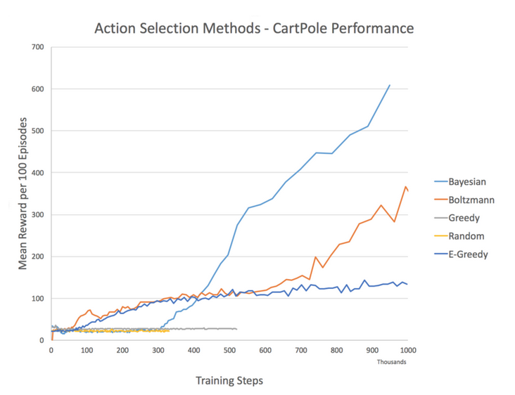
Comparison and Full Code

1.import modules

from __future__ import division

import gym
import numpy as np
import random
import tensorflow as tf
import matplotlib.pyplot as plt
%matplotlib inline

import tensorflow.contrib.slim as slim

TensorFlow-Slim

• TF-Slim is a lightweight library for defining,training and evaluating complex models in Tensorflow
• Components of tf-slim can be freely mixed with native tensorflow, as well as other frameworks, such as tf.contrib.learn

Tensorflow-Slim Usage

import tensorflow.contrib.slim as slim

Variables

weights = slim.variable('weights',
                             shape=[10, 10, 3 , 3],
                             initializer=tf.truncated_normal_initializer(stddev=0.1),
                             regularizer=slim.l2_regularizer(0.05),
                             device='/CPU:0')

Layers

input = ...
net = slim.conv2d(input, 128, [3, 3], scope='conv1_1')

Layer	TF-Slim
BiasAdd	slim.bias_add
BatchNorm	slim.batch_norm
Conv2d	slim.conv2d
Conv2dInPlane	slim.conv2d_in_plane
Conv2dTranspose (Deconv)	slim.conv2d_transpose
FullyConnected	slim.fully_connected
AvgPool2D	slim.avg_pool2d
Dropout	slim.dropout
Flatten	slim.flatten
MaxPool2D	slim.max_pool2d
OneHotEncoding	slim.one_hot_encoding
SeparableConv2	slim.separable_conv2d
UnitNorm	slim.unit_norm

def vgg16(inputs):
  with slim.arg_scope([slim.conv2d, slim.fully_connected],
                      activation_fn=tf.nn.relu,
                      weights_initializer=tf.truncated_normal_initializer(0.0, 0.01),
                      weights_regularizer=slim.l2_regularizer(0.0005)):
    net = slim.repeat(inputs, 2, slim.conv2d, 64, [3, 3], scope='conv1')
    net = slim.max_pool2d(net, [2, 2], scope='pool1')
    net = slim.repeat(net, 2, slim.conv2d, 128, [3, 3], scope='conv2')
    net = slim.max_pool2d(net, [2, 2], scope='pool2')
    net = slim.repeat(net, 3, slim.conv2d, 256, [3, 3], scope='conv3')
    net = slim.max_pool2d(net, [2, 2], scope='pool3')
    net = slim.repeat(net, 3, slim.conv2d, 512, [3, 3], scope='conv4')
    net = slim.max_pool2d(net, [2, 2], scope='pool4')
    net = slim.repeat(net, 3, slim.conv2d, 512, [3, 3], scope='conv5')
    net = slim.max_pool2d(net, [2, 2], scope='pool5')
    net = slim.fully_connected(net, 4096, scope='fc6')
    net = slim.dropout(net, 0.5, scope='dropout6')
    net = slim.fully_connected(net, 4096, scope='fc7')
    net = slim.dropout(net, 0.5, scope='dropout7')
    net = slim.fully_connected(net, 1000, activation_fn=None, scope='fc8')
  return net

Losses

import tensorflow as tf
import tensorflow.contrib.slim.nets as nets
vgg = nets.vgg

# Load the images and labels.
images, labels = ...

# Create the model.
predictions, _ = vgg.vgg_16(images)

# Define the loss functions and get the total loss.
loss = slim.losses.softmax_cross_entropy(predictions, labels)

2. Load the environment

env = gym.make('CartPole-v0')

3. Deep Q-network

class Q_Network():
    def __init__(self):
        #These lines establish the feed-forward part of the network used to choose actions

        # CartPole has 4 states -> [None,4] input
        # self.Temp is boltzmann parameter
        # self.keep_per is bayesian parameter
        self.inputs = tf.placeholder(shape=[None,4],dtype=tf.float32)
        self.Temp = tf.placeholder(shape=None,dtype=tf.float32)
        self.keep_per = tf.placeholder(shape=None,dtype=tf.float32)

        hidden = slim.fully_connected(self.inputs,64,activation_fn=tf.nn.tanh,biases_initializer=None)
        hidden = slim.dropout(hidden,self.keep_per)
        self.Q_out = slim.fully_connected(hidden,2,activation_fn=None,biases_initializer=None)
        
        self.predict = tf.argmax(self.Q_out,1)
        self.Q_dist = tf.nn.softmax(self.Q_out/self.Temp)
        
        
        #Below we obtain the loss by taking the sum of squares difference between the target and prediction Q values.
        self.actions = tf.placeholder(shape=[None],dtype=tf.int32)
        self.actions_onehot = tf.one_hot(self.actions,2,dtype=tf.float32)
        
        self.Q = tf.reduce_sum(tf.multiply(self.Q_out, self.actions_onehot), reduction_indices=1)
        
        self.nextQ = tf.placeholder(shape=[None],dtype=tf.float32)
        loss = tf.reduce_sum(tf.square(self.nextQ - self.Q))
        trainer = tf.train.GradientDescentOptimizer(learning_rate=0.0005)
        self.updateModel = trainer.minimize(loss)

-From above

# CartPole has 4 states -> [None,4] input
# self.Temp is boltzmann parameter
# self.keep_per is bayesian parameter
self.inputs = tf.placeholder(shape=[None,4],dtype=tf.float32)
self.Temp = tf.placeholder(shape=None,dtype=tf.float32)
self.keep_per = tf.placeholder(shape=None,dtype=tf.float32)

tf.reset_default_graph()

# non-statinary network 
q_net = Q_Network()
target_net = Q_Network()

init = tf.initialize_all_variables()
trainables = tf.trainable_variables()
targetOps = updateTargetGraph(trainables,tau)
myBuffer = experience_buffer()


#create lists to contain total rewards and steps per episode
jList = []
jMeans = []
rList = []
rMeans = []
with tf.Session() as sess:
    sess.run(init)
    updateTarget(targetOps,sess)
    e = startE
    stepDrop = (startE - endE)/anneling_steps
    total_steps = 0
    
    for i in range(num_episodes):
        s = env.reset()
        rAll = 0
        d = False
        j = 0
        while j < 999:
            j+=1
            if exploration == "greedy":
                #Choose an action with the maximum expected value.
                a,allQ = sess.run([q_net.predict,q_net.Q_out],\
                	feed_dict={q_net.inputs:[s],q_net.keep_per:1.0})
                a = a[0]
            if exploration == "random":
                #Choose an action randomly.
                a = env.action_space.sample()
            if exploration == "e-greedy":
                #Choose an action by greedily (with e chance of random action) from the Q-network
                if np.random.rand(1) < e or total_steps < pre_train_steps:
                    a = env.action_space.sample()
                else:
                    a,allQ = sess.run([q_net.predict,q_net.Q_out],feed_dict={q_net.inputs:[s],q_net.keep_per:1.0})
                    a = a[0]
            if exploration == "boltzmann":
                #Choose an action probabilistically, with weights relative to the Q-values.
                Q_d,allQ = sess.run([q_net.Q_dist,q_net.Q_out],feed_dict={q_net.inputs:[s],q_net.Temp:e,q_net.keep_per:1.0})
                a = np.random.choice(Q_d[0],p=Q_d[0])
                a = np.argmax(Q_d[0] == a)
            if exploration == "bayesian":
                #Choose an action using a sample from a dropout approximation of a bayesian q-network.
                a,allQ = sess.run([q_net.predict,q_net.Q_out],feed_dict={q_net.inputs:[s],q_net.keep_per:(1-e)+0.1})
                a = a[0]
                
            ...

• Greedy policy

if exploration == "greedy":
    #Choose an action with the maximum expected value.
    a,allQ = sess.run([q_net.predict,q_net.Q_out],\
    	feed_dict={q_net.inputs:[s],q_net.keep_per:1.0})
    a = a[0]
    # a is greedy value from self.predict, self.predict choose the argmax action values
...

class Q_Network():
    ...
    # self.Q_out is Network output from fully connected layer
	self.Q_out = slim.fully_connected(hidden,2,activation_fn=None,biases_initializer=None)
    # self.predcit is argmax from self.Q_out
	self.predict = tf.argmax(self.Q_out,1)
    ...

q_net = Q_Network()
print(q_net.Q_out,q_net.predict)
>>  Tensor("fully_connected_1/MatMul:0", shape=(?, 2), dtype=float32) Tensor("ArgMax:0", shape=(?,), dtype=int64)

• e-Greedy policy

if exploration == "e-greedy":
    #Choose an action by greedily (with e chance of random action) from the Q-network
    if np.random.rand(1) < e or total_steps < pre_train_steps:
        a = env.action_space.sample() # random action 
    else: # greedy policy
        a,allQ = sess.run([q_net.predict,q_net.Q_out],\
            feed_dict={q_net.inputs:[s],q_net.keep_per:1.0})
        a = a[0]

• boltzmann policy

startE = 1 #Starting chance of random action
e = startE
# weighted policy on each actions
if exploration == "boltzmann":
    #Choose an action probabilistically, with weights relative to the Q-values.
    Q_d,allQ = sess.run([q_net.Q_dist,q_net.Q_out]\
        ,feed_dict={q_net.inputs:[s],q_net.Temp:e,q_net.keep_per:1.0})
    a = np.random.choice(Q_d[0],p=Q_d[0])
    a = np.argmax(Q_d[0] == a)

# e is temp parameter
# self.Q_dist is softmax output
class Q_Network():
    self.Q_out = slim.fully_connected(hidden,2,activation_fn=None,biases_initializer=None)
    self.Q_dist = tf.nn.softmax(self.Q_out/self.Temp)

• bayesian policy

startE = 1 #Starting chance of random action
endE = 0.1 #Final chance of random action
anneling_steps = 200000 #How many steps of training to reduce startE to endE.
pre_train_steps = 50000 #Number of steps used before training updates begin.

stepDrop = (startE - endE)/anneling_steps
...

if exploration == "bayesian":
    #Choose an action using a sample from a dropout approximation of a bayesian q-network.
    a,allQ = sess.run([q_net.predict,q_net.Q_out]\
        ,feed_dict={q_net.inputs:[s],q_net.keep_per:(1-e)+0.1})
    a = a[0]
...
if e > endE and total_steps > pre_train_steps:
    e -= stepDrop
...

class Q_Network:

    self.Q_out = slim.fully_connected(hidden,2,activation_fn=None,biases_initializer=None)    
    self.predict = tf.argmax(self.Q_out,1)

Reference sites

Simple Reinforcement Learning with Tensorflow Part 7: Action-Selection Strategies for Exploration

Deep Reinforcement Learning Agents

This repository contains a collection of reinforcement learning algorithms written in Tensorflow. The ipython notebook here were written to go along with a still-underway tutorial series I have been publishing on Medium. If you are new to reinforcement learning, I recommend reading the accompanying post for each algorithm.

The repository currently contains the following algorithms:

• Q-Table - An implementation of Q-learning using tables to solve a stochastic environment problem.
• Q-Network - A neural network implementation of Q-Learning to solve the same environment as in Q-Table.
• Simple-Policy - An implementation of policy gradient method for stateless environments such as n-armed bandit problems.
• Contextual-Policy - An implementation of policy gradient method for stateful environments such as contextual bandit problems.
• Policy-Network - An implementation of a neural network policy-gradient agent that solves full RL problems with states and delayed rewards, and two opposite actions (ie. CartPole or Pong).
• Vanilla-Policy - An implementation of a neural network vanilla-policy-gradient agent that solves full RL problems with states, delayed rewards, and an arbitrary number of actions.
• Model-Network - An addition to the Policy-Network algorithm which includes a separate network which models the environment dynamics.
• Double-Dueling-DQN - An implementation of a Deep-Q Network with the Double DQN and Dueling DQN additions to improve stability and performance.
• Deep-Recurrent-Q-Network - An implementation of a Deep Recurrent Q-Network which can solve reinforcement learning problems involving partial observability.
• Q-Exploration - An implementation of DQN containing multiple action-selection strategies for exploration. Strategies include: greedy, random, e-greedy, Boltzmann, and Bayesian Dropout.
• A3C-Doom - An implementation of Asynchronous Advantage Actor-Critic (A3C) algorithm. It utilizes multiple agents to collectively improve a policy. This implementation