t-SNE

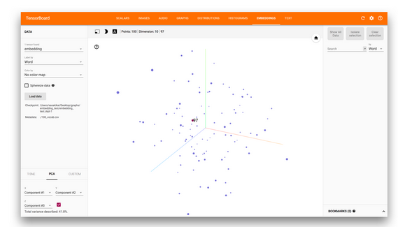
t-SNE visualization by TensorFlow

• From Tensorflow 0.12, it provides the functionality for visualizing embedding space of data samples.
• It is useful for checking the cluster in embedding by your eyes
• Embedding means the way to project a data into the distributed representation in a space
• This technique is used NLP method and famous by word2vec
• We have a word dictionary which is encoded in one-hot style
  
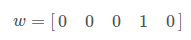
• w represents a word 4th indexed in the dictionary
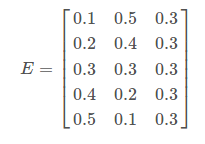
• And we have embedding matrix which can try to convert a word dictionary into 3 dimension embedding space
  
• By multiplying them, we have a distributed representation of the word w
  
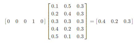
  • Provides useful information about the relationship between each words
  • Avoid sparse dataset which often require more data to make model more accurate
• Converting a word into such continuous vector space is an useful technique
• Embedding matrix can be obtained through the process like word2vec
• In this post, we tried to write a minimal code to visualize the embedding space with given embedding matrix
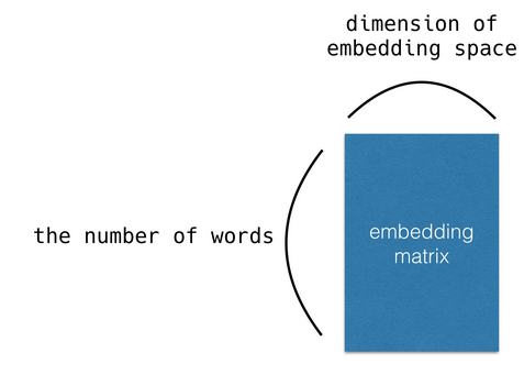
• we can visualize any 2 dimensional matrix but the format should be like this
  
• So first we try to create the dummy embedding matrix with random

import tensorflow as tf
embedding_var = tf.Variable(tf.truncated_normal([100, 10]), name='embedding')

• In this case, we assume that we have 100 words and it can be converted into 10 dimension space. Please make sure embedding_var is made as Variable

Then we visualize this

from tensorflow.contrib.tensorboard.plugins import projector

with tf.Session() as sess:
    # Create summary writer.
    writer = tf.summary.FileWriter('./graphs/embedding_test', sess.graph)
    # Initialize embedding_var
    sess.run(embedding_var.initializer)
    # Create Projector config
    config = projector.ProjectorConfig()
    # Add embedding visualizer
    embedding = config.embeddings.add()
    # Attache the name 'embedding'
    embedding.tensor_name = embedding_var.name
    # Metafile which is described later
    embedding.metadata_path = './100_vocab.csv'
    # Add writer and config to Projector
    projector.visualize_embeddings(writer, config)
    # Save the model
    saver_embed = tf.train.Saver([embedding_var])
    saver_embed.save(sess, './graphs/embedding_test/embedding_test.ckpt', 1)

writer.close()

• Summary writer writes a file including necessary information to visualize
• It is used by TensorBoard later
• Meta file is used for showing additional data to each words such as word string
• Its format should be csv and indexed same as embedding matrix
• For example, if we have a word “apple” in 5th position in embedding matrix, the word should also positioned 5th line in 100_vocab.csv

TensorBoard

• TensorBoard is a tool for visualizing embedding space.

  tensorboard --logdir=graphs/embedding_test
  

---

---

---

Classifying and visualizing with fastText and tSNE

Methods

• (1) A representation of a block of text
• (2) A classifier based on that representation

• (3) Visualization method

• (1) and (2) are similar
• For a classifier I used fastText
• This method treates a block of text as a bag of word vectors
  • it learns word vectors based on the corpus(which is done using an unsupervised deep neural network)
  • the bag of words model works surprisingly well
• For visualization it again use the tSNE algorithm,
  • The scikit-learn implementation of tSNE transforms one specific dataset
  • The parametric tSNE algorithm trains a neural network using an appropriate cost function, meaning new points can be transformed from the high-dimensional space to the low-dimensional space
• It implemented this in Tensorflow and the newly incorporated tf.contrib.keras functionality

jsilter/parametric_tsne

parametric_tsne Overview

This is a python package implementing parametric t-SNE. We train a neural-network to learn a mapping by minimizing the Kullback-Leibler divergence between the Gaussian distance metric in the high-dimensional space and the Students-t distributed distance metric in the low-dimensional space. By default we use similar archictecture1 as van der Maaten 2009, which is a dense neural network with layers: [input dimension], 500, 500, 2000, [output dimension]

Results

• tSNE of all 14 dbPedia classes
  
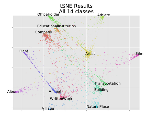
  • In contrast expectation from methods like PCA, classes which we expect to be similar don’t get placed closer together
  • The Plant and Animal cluster are distant, and Animal is closer to WrittenWork
  • Company,EducationalInstitution, and OfficeHolder are all near each other
  • There is an extremely mild correlation between the clusters but if placement were done by correlation, Plant and Animal would be right next to each other
  • There is evidence of that similarity in a different way
  • Many Plant and Animal points lie on a line running directly from one cluster to another
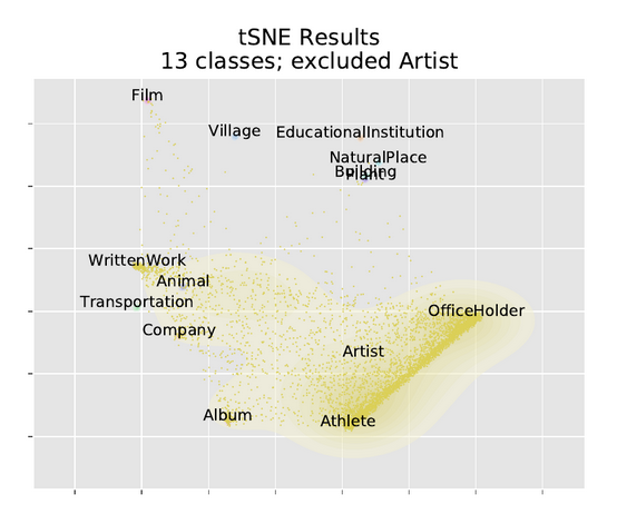
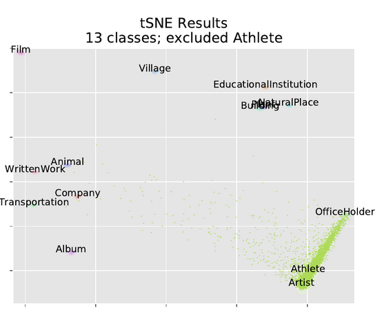
• tSNE excluding single classes
  • excluding 1 class each time, building a model with 13 outputs instead of 14
  • Then running the excluded class through the model, we see how members of the excluded class get clustered
  • we visulaize using our parametric tSNE, and also a joy plot of the log probability of each class
  • In these tSNE plots we only plotted scattered points for the excluded class
    

---

---

---

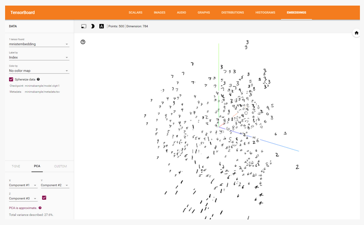
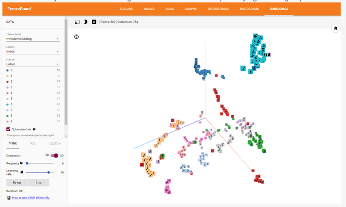
Simple Introduction to Tensorboard Embedding Visualisation

• Embedding visualization is a standard feature in Tensorboard
• visualization of MNIST digits runnning

%matplotlib inline
import matplotlib.pyplot as plt
import tensorflow as tf
import numpy as np
import os

from tensorflow.contrib.tensorboard.plugins import projector
from tensorflow.examples.tutorials.mnist import input_data

LOG_DIR = 'minimalsample'
NAME_TO_VISUALISE_VARIABLE = "mnistembedding"
TO_EMBED_COUNT = 500


path_for_mnist_sprites =  os.path.join(LOG_DIR,'mnistdigits.png')
path_for_mnist_metadata =  os.path.join(LOG_DIR,'metadata.tsv')

What to visualize

• Although the embedding visualiser is meant for visualising embedding obtained after training, you can also use it to apply visualization of normal MNIST digits
• each digit is represented by a vector with length 28 * 28=784 dimensions

mnist = input_data.read_data_sets("MNIST_data/", one_hot=False)
batch_xs, batch_ys = mnist.train.next_batch(TO_EMBED_COUNT)

Creating the embeddings

• the name of the variable

  embedding_var = tf.Variable(batch_xs, name=NAME_TO_VISUALISE_VARIABLE)
  summary_writer = tf.summary.FileWriter(LOG_DIR)
  

Creating the embedding projector

• This is important part of visualization
• you specify what variable you want to project, what metadata path path is(the name and classes), and where you save the sprites

config = projector.ProjectorConfig()
embedding = config.embeddings.add()
embedding.tensor_name = embedding_var.name

# Specify where you find the metadata
embedding.metadata_path = path_for_mnist_metadata #'metadata.tsv'

# Specify where you find the sprite (we will create this later)
embedding.sprite.image_path = path_for_mnist_sprites #'mnistdigits.png'
embedding.sprite.single_image_dim.extend([28,28])

# Say that you want to visualise the embeddings
projector.visualize_embeddings(summary_writer, config)

Saving the data

• Tensorboard loads the saved variable from the saved graph, initialize a session and variables and save them in your logging directory

sess = tf.InteractiveSession()
sess.run(tf.global_variables_initializer())
saver = tf.train.Saver()
saver.save(sess, os.path.join(LOG_DIR, "model.ckpt"), 1)

Visualization helper functions

• If you don’t load sprites each digit is represented as a simple point

• To add labels you have to create a ‘sprite map’

  • create_sprite_image: neatly aligns image sprites on a square canvas
  • vector_to_matrix_mnist: MNIST characters are loaded as a vector, not as an image, this function turns them into images
  • invert_grayscale:matplotlib treats a 0 as black and 1 as a white

def create_sprite_image(images):
    """Returns a sprite image consisting of images passed as argument. Images should be count x width x height"""
    if isinstance(images, list):
        images = np.array(images)
    img_h = images.shape[1]
    img_w = images.shape[2]
    n_plots = int(np.ceil(np.sqrt(images.shape[0])))
    
    
    spriteimage = np.ones((img_h * n_plots ,img_w * n_plots ))
    
    for i in range(n_plots):
        for j in range(n_plots):
            this_filter = i * n_plots + j
            if this_filter < images.shape[0]:
                this_img = images[this_filter]
                spriteimage[i * img_h:(i + 1) * img_h,
                  j * img_w:(j + 1) * img_w] = this_img
    
    return spriteimage

def vector_to_matrix_mnist(mnist_digits):
    """Reshapes normal mnist digit (batch,28*28) to matrix (batch,28,28)"""
    return np.reshape(mnist_digits,(-1,28,28))

def invert_grayscale(mnist_digits):
    """ Makes black white, and white black """
    return 1-mnist_digits

Save the sprite image

to_visualise = batch_xs
to_visualise = vector_to_matrix_mnist(to_visualise)
to_visualise = invert_grayscale(to_visualise)

sprite_image = create_sprite_image(to_visualise)

plt.imsave(path_for_mnist_sprites,sprite_image,cmap='gray')
plt.imshow(sprite_image,cmap='gray')

Save the metadata

• To add colors to your mnist digits, the embedding visualization tool needs to know what label each image has
• the index is simply the index in our embedding matrix
• the label is the label of the MNIST character

with open(path_for_mnist_metadata,'w') as f:
    f.write("Index\tLabel\n")
    for index,label in enumerate(batch_ys):
        f.write("%d\t%d\n" % (index,label))

How to run

tensorboard --logdir=minimalsample

Tutorial

t-SNE visualization by TensorFlow

Classifying and visualizing with fastText and tSNE

Simple Introduction to Tensorboard Embedding Visualisation