Hvass Time series prediction
Introduction
- This Tutorial tries to predict the future weather of a city using weather data from several other cities
- We will use a Recurrent Neural Network(RNN)
Data
- weather data from the period 1980-2018 for five cities in Denmark
- Aalborg The weather-data is actually from an airforce base which is also home to [The Hunter Corps (Jægerkorps)](https://en.wikipedia.org/wiki/Jaeger_Corps_(Denmark).
- Aarhus is the city where the inventor of C++ studied and the Google V8 JavaScript Engine was developed.
- Esbjerg has a large fishing-port.
- Odense is the birth-city of the fairytale author H. C. Andersen.
- Roskilde has an old cathedral housing the tombs of the Danish royal family.
Flowchart
- we are trying to predict the weather for the Odense 24 hours into the future
- given the current and past weather data from 5 cities
- we use a RNN because it can work on sequences of arbitrary length
- During training we will use sequences of 100 data points from the training-set, with each data point or observation having 20 input signals for the temperature, pressure, etc
- we want to train the NN so it outputs the 3 signals for tomorrow’s temperature, pressure, and wind-speed

Imports
%matplotlib inline
import matplotlib.pyplot as plt
import tensorflow as tf
import numpy as np
import pandas as pd
import os
from sklearn.preprocessing import MinMaxScaler

# from tf.keras.models import Sequential  # This does not work!
from keras.models import Sequential
from keras.layers import Input, Dense, GRU, Embedding
from keras.optimizers import RMSprop
from keras.callbacks import EarlyStopping, ModelCheckpoint, TensorBoard

import h5py
Load Data
import weather
weather.maybe_download_and_extract()
cities = weather.cities
cities
>> ['Aalborg', 'Aarhus', 'Esbjerg', 'Odense', 'Roskilde']
- save the data in the cache so it loads very quickly the next time
df.to_pickle(path)
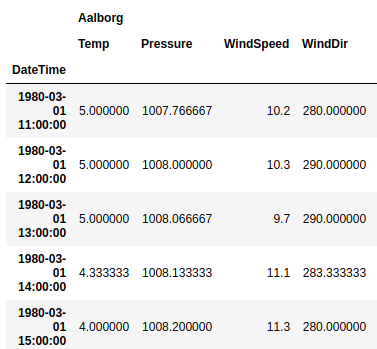
df.head()
df['Esbjerg']['Pressure'].plot()
df['Roskilde']['Pressure'].plot()
df.values.shape
>> (333109,20)
- drop missing data in the columns
df.drop(('Esbjerg', 'Pressure'), axis=1, inplace=True)
df.drop(('Roskilde', 'Pressure'), axis=1, inplace=True)
df.values.shape
>>(333109,18)
Data Errors
- There are some errors in this data. As shown in the plot below, the temperature in the city of Odense suddenly jumped to almost 50 degrees C. But the highest temperature ever measured in Denmark was only 36.4 degrees Celcius and the lowest was -31.2 C. So this is clearly a data error. However, we will not correct any data-errors in this tutorial.
df['Odense']['Temp']['2006-05':'2006-07'].plot()
Add Data
We can add some input-signals to the data that may help our model in making predictions.
For example, given just a temperature of 10 degrees Celcius the model wouldn’t know whether that temperature was measured during the day or the night, or during summer or winter. The model would have to infer this from the surrounding data-points which might not be very accurate for determining whether it’s an abnormally warm winter, or an abnormally cold summer, or whether it’s day or night. So having this information could make a big difference in how accurately the model can predict the next output.
Although the data-set does contain the date and time information for each observation, it is only used in the index so as to order the data. We will therefore add separate input-signals to the data-set for the day-of-year (between 1 and 366) and the hour-of-day (between 0 and 23).
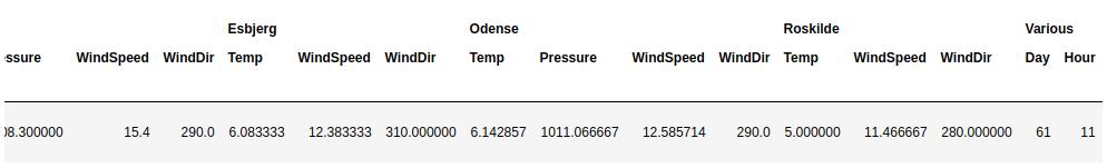
df['Various', 'Day'] = df.index.dayofyear
df['Various', 'Hour'] = df.index.hour
df.head()

Target Data for Prediction
predict the future weather data for this city
target_city = 'Odense'
target_names = ['Temp', 'WindSpeed', 'Pressure']

shift_days = 1
shift_steps = shift_days * 24  # Number of hours.

df_targets = df[target_city][target_names].shift(shift_steps)
NumPy Arrays
We now convert the Pandas data-frames to NumPy arrays that can be input to the neural network. We also remove the first part of the numpy arrays, because the target-data has NaN for the shifted period, and we only want to have valid data and we need the same array-shapes for the input- and output-data.
x_data = df.values[shift_steps:]
y_data = df_targets.values[shift_steps:]

train_split = 0.9
num_train = int(train_split * num_data)

num_test = num_data - num_train

x_train = x_data[0:num_train]
x_test = x_data[num_train:]
len(x_train) + len(x_test)

y_train = y_data[0:num_train]
y_test = y_data[num_train:]
len(y_train) + len(y_test)

num_x_signals = x_data.shape[1]
num_x_signals
>> 20
num_y_signals = y_data.shape[1]
num_y_signals
Scaled Data
The data-set contains a wide range of values
- normalization with MinMaxScaler
print("Min:", np.min(x_train))
print("Max:", np.max(x_train))
>>Min: -27.0
>>Max: 1050.8

x_scaler = MinMaxScaler()
x_train_scaled = x_scaler.fit_transform(x_train)

print("Min:", np.min(x_train_scaled))
print("Max:", np.max(x_train_scaled))

>>Min: 0.0
>>Max: 1.0000000000000002

x_test_scaled = x_scaler.transform(x_test)
y_scaler = MinMaxScaler()
y_train_scaled = y_scaler.fit_transform(y_train)
y_test_scaled = y_scaler.transform(y_test)
Data Generator
The data-set has now been prepared as 2-dimensional numpy arrays. The training-data has almost 300k observations, consisting of 20 input-signals and 3 output-signals.
These are the array-shapes of the input and output data:
print(x_train_scaled.shape)
print(y_train_scaled.shape)
>>(299776, 20)
>>(299776, 3)
But the Recurrent Neural Network cannot be trained on sequences with 300k observations. **RNN is only trained on small sequences of e.g. 100 observations. **Furthermore, in order to improve the training-efficiency when using a GPU, we will use batches of training-data.
For example, we may want a random batch of 1024 sequences, with each sequence having 100 observations, and each observation having 20 input-signals and 3 output-signals.
This function generates such random batches of data.
batch_size = 1024
sequence_length = 100
generator = batch_generator(batch_size=batch_size,
                            sequence_length=sequence_length)

batch = 0   # First sequence in the batch.
signal = 9  # First signal out of the 20 input-signals.
seq = x_batch[batch, :, signal]
plt.plot(seq)

seq = y_batch[batch, :, signal]
plt.plot(seq)
Validation Set
validation_data = (np.expand_dims(x_test_scaled, axis=0),
                   np.expand_dims(y_test_scaled, axis=0))

validation_data[0].shape
>> (1, 33309, 20)
Create the Recurrent Neural Network
- The output-signals in the data-set have been limited to be between 0 and 1 using a
scaler-object. So we also limit the output of the neural network using the Sigmoid activation function, which squashes the output to be between 0 and 1. -
MinMaxScaler() normalizes the scalar value between 0 and 1
- We will use Mean Squared Error (MSE) as the loss-function that will be minimized.
This measures how closely the model’s output matches the true output signals.
model = Sequential()

model.add(GRU(units=256,
              return_sequences=True,
              input_shape=(None, num_x_signals,)))

model.add(Dense(num_y_signals, activation='sigmoid'))

optimizer = RMSprop(lr=1e-3)

model.compile(loss='mean_squared_error',
              optimizer=optimizer,
              metrics=['mae'])
Callback Functions
path_checkpoint = '23_checkpoint.keras'
callback_checkpoint = ModelCheckpoint(filepath=path_checkpoint,
                                      monitor='val_loss',
                                      verbose=1,
                                      save_weights_only=True,
                                      save_best_only=True)

callback_early_stopping = EarlyStopping(monitor='val_loss',
                                        patience=5, verbose=1)

callback_tensorboard = TensorBoard(log_dir='./23_logs/',
                                   histogram_freq=0,
                                   write_graph=False)
callbacks = [callback_early_stopping,
             callback_checkpoint,
             callback_tensorboard]
Train the Recurrent Neural Network
steps_per_epoch = int(num_train / batch_size)
steps_per_epoch

%%time
model.fit_generator(generator=generator,
                    epochs=3,#20,
                    steps_per_epoch=steps_per_epoch,
                    validation_data=validation_data,
                    callbacks=callbacks)
python KL divergence
import numpy as np

def KL(P,Q):
""" Epsilon is used here to avoid conditional code for
checking that neither P nor Q is equal to 0. """
     epsilon = 0.00001

     # You may want to instead make copies to avoid changing the np arrays.
     P = P+epsilon
     Q = Q+epsilon

     divergence = np.sum(P*np.log(P/Q))
     return divergence

# Should be normalized though
values1 = np.asarray([1.346112,1.337432,1.246655])
values2 = np.asarray([1.033836,1.082015,1.117323])

# Note slight difference in the final result compared to Dawny33
print KL(values1, values2) # 0.775278939433
KL divergence between two univariate Gaussians
KL divergence between two univariate Gaussians
- KL(p, q) = \log \frac{\sigma_2}{\sigma_1} + \frac{\sigma_1^2 + (\mu_1 - \mu_2)^2}{2 \sigma_2^2} - \frac{1}{2}