Predict Stock Price using RNN
Introduction
- This tutorial is for how to build a recurrent neural network using Tensorflow to predict stock market prices
- Part 1 focuses on the prediction of S$P 500 index
- This motivation is demonstrating how to build and train on RNN model in Tensorflow and less on solve the stock prediction problem
Recurrent Neural Network
- A sequence model is usually designed to transform an input sequence into an output sequence that lives in a different domain
- RNN shows us tremendous improvement in handwriting recognition,speech recognition, and machine translation
- A RNN model is born with the capability to process long sequential data and to tackle with context spreading in time
- Imagine the case when an RNN model reads all the Wikipedia articles, character by character, and then it can predict the following words given the context
-
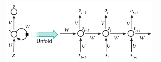
- However,simple perception neurons that linearly combine the current input and the last unit state may easily lose the long-term dependencies
- For example, we start a sentence with “Alice is working at…” and later after a whole paragraph, we want to start the next sentence with “She” or “He” correctly
- If the model forgets the character’s name “Alice”,we can never know
- To resolve the issue, researchers created a special neuron with a much more complicated internal structure for memorizing long-ternm context, named Long short tern memory(LSTM)
- It is smart enough to learn for how long it should memorize the old information, when to forget, when to make sure of the new data, and how to combine the old memory with new input
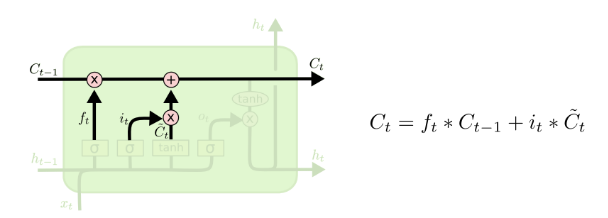
LSTM networks
- LSTM is a special kind of RNN
- LSTM are explicitly designed to avoid the long-term dependency problem
- Remembering information for long periods of time is practically their default behavior
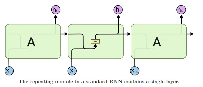
- LSTM also have this chain structure but the repeating module has a different structure
- Instead of having a single neural network layer, there are four structure
-
LSTM repeating module contains four interacting layers
- each line carries an entire vector: from the output of one node to the input of others
- The Pink circles represent pointwise operation like vector addition
- the yellow boxes are learned neural network layers
- Line merging denote concatenation
- a line forking denote a content being copied and the copies going to different locations
Core Idea Behind LSTM
- The key to LSTMs is the cell state, the horizonal line running through the top of the diagram
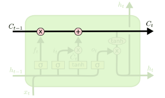
- The LSTM does have the ability to remove or add information to the cell state, carefully regulated by structures called gates
- Gates are a way to optionally let information through
- They are composed out of a sigmoid neural net layer between zero and one and a pointwise multiplication operation
- sigmoid output[0,1] means how much of each component should be let through
- A zero means let nothing through
- A one means let everything through
- A LSTM has threee gates to protect and control the cell state
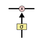
Step by Step LSTM Walk Through
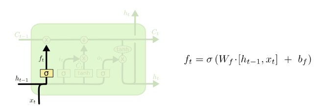
- The first step in our LSTM is to decide what information we’re going to throw away from the cell state
- This decision is made by a sigmoid layer called the “forget gate layer”
- It looks at
 and
and  and outputs a number between 0 and 1 for each number in the cell state
- 1 represents completely keep this while 0 represents get rid of this
- Let’s go back to our example of a language model trying to predict the next word based on all the previous ones
- In such a problem, the cell state might include the gender of the present subject, so that the correct pronouns can be used
- When we see a new subject, we want to forget the gender of the old subject
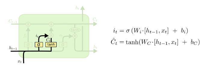
- The Next step is to decide what new information we’re going to store in the cell state
- This has two parts
- First, a sigmoid layer called “input gate layer” decides which values we’ll update
- Next, a tanh layer creates a vector of new candidate values,
 that could be added to the state
 - In the next step, we’ll combine these two to create an update to the state
- In the example of our language model, we’d want to add the gender of the new subject to the cell state, to replace the old one we’re forgetting
-
- It’s now time to update the old cell state,
 , into the new cell state
- We multiply the old state by
 , forgetting the things we decided to forget earlier
 - Then we add
 , This is the new candidate values, scaled by how much we decided to update each state value
 - In the case of language model, this is where we’d actually drop the information about the old subject’s gender and add the new information
- Finally, we need to decide what we’re goint to output
- This output will be based on our cell state, but will be a filtered version
- First, we run a sigmoid layer which decides what parts of the cell state we’re going to output
- Then, we put the cell state through tanh(to push the values to be between -1 and 1) and multiply it by the output of the sigmoid gate,so that we only output the parts we decided to
- for language model,since it just saw a subject, it might want to output information relevant to a verb, in case that’s what is coming next
- For example, it might output whether the subject is singular or plural,so that we know what form a verb should be conjugated into if that’s what follows next
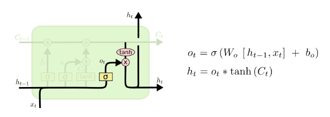
- This output will be based on our cell state, but will be a filtered version
Overview
- use Penn Tree Bank(PTB) datasets
- PTB show a RNN model in a pretty and modular design pattern
The Goal
- explain how to build an RNN model with LSTM cells to predict the prices
- The dataset can be downloaded from Yahoo
- data from Jan 3,1950 to Jun 23,2017
- The dataset provides several price points per day
- we just use the daily close prices for prediction
- demonstrate how to use TensorBoard for easily debugging and model tracking
- RNN uses the previous state of the hidden neuron to learn the current state given the new input
- RNN is good at processing sequential data
- LSTM helps RNN better memorize the long-term context
Data Preparation
- The stock price is a time series of length N, defined
 in which
  is the close price on day
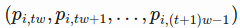
 - we have a sliding window of a fixed size
 (input_size)
 - every time we move the window to the right by size , so that there is no overlap between data in all the sliding windows
-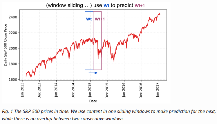
- RNN model we are about to build has LSTM cells as basic hidden units
- We use values from the beginning in the first sliding window
 to the window
  at time t
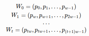
- to predict the prices in the following window

- Essentially we try to learn an approximation function
- We use values from the beginning in the first sliding window
-
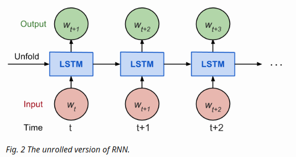
- Considering how back propagation throught time works, we usually train RNN in a unrolled version so that we don’t have to do propagation computation too far back and save the training complication
- Here is the explanation on num_steps from Tensorflow’s tutorial
By design, the output of a RNN depends on arbitrarily distant inputs. Unfortunately, this makes backpropagation computation difficult. In order to make the learning process tractable, it is common practice to create an “unrolled” version of the network, which contains a fixed number(num_steps) of LSTM inputs and outputs. The model is then trained on this finite approximation of the RNN. This can be implemented by feeding inputs of length num_steps at a time and performing a backward pass after each such input block
- The sequences of prices are first split into non-overlapped small windows
- Each contains input_size numbers and each is considered as one independent input element
- Then num_steps consecutive input elements are grouped into one training input, forming an “unrolled” version of RNN for training on Tensorflow
- for instance, if input_size = 3 and num_steps = 2, training examples would look like
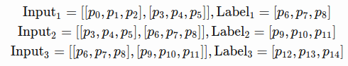
seq = [np.array(seq[i * self.input_size: (i + 1) * self.input_size])
       for i in range(len(seq) // self.input_size)]

# Split into groups of `num_steps`
X = np.array([seq[i: i + self.num_steps] for i in range(len(seq) - self.num_steps)])
y = np.array([seq[i + self.num_steps] for i in range(len(seq) - self.num_steps)])

import numpy as np
input_size = 3
num_steps = 2

seq = [0,1,2,3,4,5,6,7,8,9]
seq = [np.array(seq[i * input_size: (i + 1) * input_size])
       for i in range(len(seq) // input_size)]

seq
Out[2]:
[array([0, 1, 2]), array([3, 4, 5]), array([6, 7, 8])]

X = np.array([seq[i: i + num_steps] for i in range(len(seq) - num_steps)])
X
Out[4]
array([[[0, 1, 2],
        [3, 4, 5]]])

len(seq) - num_steps
Out[5]
1
Train/Test Split
- Since we want to predict the future, we take the latest 10% of data as the test data
Normalization
- The S&P 500 index increases in time, bringing about the problem that most values in the test set are out of the scale of the train set
- thus the model has to predict some numbers it has never seen before
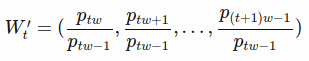
- To solve the out of scale issue, I normalize the prices in each sliding window
- The task becomes predicting the relative change rates instead of the absolute values
- In a normalized sliding window
 at time t, all values are divided by the last unknown price- the last price in
Model Construction
- Definitions
- lstm_size: number of units in one LSTM layer
- num_layers : number of stacked LSTM layers
- keep_prob: percentage of cell units to keep in the dropout operation
- init_learning_rate: the learning rate to start with
- learning_rate_decay : decay ratio in later training epochs
- init_epoch: total number of epochs in training
- input_size: size of the sliding window/ one training data point
- batch_size: number of data points to use in one-mini batch
# Configuration is wrapped in one object for easy tracking and passing.
class RNNConfig():
    input_size=1
    num_steps=30
    lstm_size=128
    num_layers=1
    keep_prob=0.8
    batch_size = 64
    init_learning_rate = 0.001
    learning_rate_decay = 0.99
    init_epoch = 5
    max_epoch = 50

config = RNNConfig()
Define Graph
- A tf.Graph is not attached to any real data
- It defines the flow of how to process the data and how to run the computation
- later, this graph can be fed with data within a tf.session and at this moment the computation happens for real
(1) Initialize a new graph first
import tensorflow as tf
tf.reset_default_graph()
lstm_graph = tf.Graph()
(2) How the graph works within its scope
with lstm_graph.as_default():
(3) Define the data required for computation Here we need three inputs, all defined as tf.placeholder because we don’t know what they are at the graph construction stage
- inputs: the training data X, a tensor of shape(# data examples, num_steps, input_size), the number of data examples is unknown,so it is None.
- targets: the training label y, a tensor of shape(#data example, input_size)
- learning_rate: a simple float
# Dimension = (
#     number of data examples,
#     number of input in one computation step,
#     number of numbers in one input
# )
# We don't know the number of examples beforehand, so it is None.
inputs = tf.placeholder(tf.float32, [None, config.num_steps, config.input_size])
targets = tf.placeholder(tf.float32, [None, config.input_size])
learning_rate = tf.placeholder(tf.float32, None)
(4) This function returns one LSTMCell with or without dropout operation
def _create_one_cell():
        return tf.contrib.rnn.LSTMCell(config.lstm_size, state_is_tuple=True)
        if config.keep_prob < 1.0:
            return tf.contrib.rnn.DropoutWrapper(lstm_cell, output_keep_prob=config.keep_prob)
(5) Let’s stack the cells into multiple layers if needed. MultiRNNCell helps connect sequentially multiple simple cells to compose one cell
    cell = tf.contrib.rnn.MultiRNNCell(
        [_create_one_cell() for _ in range(config.num_layers)],
        state_is_tuple=True
    ) if config.num_layers > 1 else _create_one_cell()
(6) tf.nn.dynamic_rnn constructs a recurrent neural network specified by cell (RNNCell). It returns a pair of (model outpus, state), where the outputs val is of size (batch_size, num_steps, lstm_size) by default. The state refers to the current state of the LSTM cell, not consumed here
val, _ = tf.nn.dynamic_rnn(cell, inputs, dtype=tf.float32)
(7) tf.transpose converts the outputs from the dimension (batch_size, num_steps, lstm_size) to (num_steps, batch_size, lstm_size). Then the last output is picked
    # Before transpose, val.get_shape() = (batch_size, num_steps, lstm_size)
    # After transpose, val.get_shape() = (num_steps, batch_size, lstm_size)
    val = tf.transpose(val, [1, 0, 2])
    # last.get_shape() = (batch_size, lstm_size)
    last = tf.gather(val, int(val.get_shape()[0]) - 1, name="last_lstm_output")
(8) Define weights and biases between the hidden and output layers
weight = tf.Variable(tf.truncated_normal([config.lstm_size, config.input_size]))
bias = tf.Variable(tf.constant(0.1, shape=[config.input_size]))
prediction = tf.matmul(last, weight) + bias
(9) We use mean square error as the loss metric and the RMSPropOptimizer algorithm for gradient descent optimization
    loss = tf.reduce_mean(tf.square(prediction - targets))
    optimizer = tf.train.RMSPropOptimizer(learning_rate)
    minimize = optimizer.minimize(loss)
Start Training Session
with tf.Session(graph=lstm_graph) as sess:
  ...
  tf.global_variables_initializer().run()
  ...
  for epoch_step in range(config.max_epoch):
        current_lr = learning_rates_to_use[epoch_step]

        # Check https://github.com/lilianweng/stock-rnn/blob/master/data_wrapper.py
        # if you are curious to know what is StockDataSet and how generate_one_epoch()
        # is implemented.
        for batch_X, batch_y in stock_dataset.generate_one_epoch(config.batch_size):
            train_data_feed = {
                inputs: batch_X,
                targets: batch_y,
                learning_rate: current_lr
            }
            train_loss, _ = sess.run([loss, minimize], train_data_feed)
  ...

  saver = tf.train.Saver()
  saver.save(sess, "your_awesome_model_path_and_name", global_step=max_epoch_step)
  ...
Use TensorBoard
Brief Summary
- Use with [tf.name_scope]: to wrap elements working on the similar goal together
- Many tf.* methods accepts name= argument. Assigning a customized name can make your life much easier
- tf.summary.scalar and tf.summary.histogram help track the values of variables in the graph during iterations
- In the training session, define a log file using tf.summary.FileWriter
with tf.Session(graph=lstm_graph) as sess:
    merged_summary = tf.summary.merge_all()
    writer = tf.summary.FileWriter("location_for_keeping_your_log_files", sess.graph)
    writer.add_graph(sess.graph)
Later, write the training progress and summary results into the file
_summary = sess.run([merged_summary], test_data_feed)
writer.add_summary(_summary, global_step=epoch_step)  # epoch_step in range(config.max_epoch)
Results
- configuration
num_layers=1
keep_prob=0.8
batch_size = 64
init_learning_rate = 0.001
learning_rate_decay = 0.99
init_epoch = 5
max_epoch = 100
num_steps=30
Handling Multiple Stock Data
- In order to distinguish the patterns associated with different price sequences
- It use the stock symbol embedding vectors as part of the input
Dataset
- data fetch codes
import urllib2
from datetime import datetime
BASE_URL = "https://www.google.com/finance/historical?"
           "output=csv&q={0}&startdate=Jan+1%2C+1980&enddate={1}"
symbol_url = BASE_URL.format(
    urllib2.quote('GOOG'), # Replace with any stock you are interested.
    urllib2.quote(datetime.now().strftime("%b+%d,+%Y"), '+')
)

try:
    f = urllib2.urlopen(symbol_url)
    with open("GOOG.csv", 'w') as fin:
        print >> fin, f.read()
except urllib2.HTTPError:
    print "Fetching Failed: {}".format(symbol_url)
Model Construction
- The model is expected to learn the price sequences of different stocks in time
- Due to the different underlying patterns, I would like to tell the model which stock it is dealing with
- Embedding is more favored than one-hot encoding
In mathematics, an embedding (or imbedding[1]) is one instance of some mathematical structure contained within another instance, such as a group that is a subgroup. When some object X is said to be embedded in another object Y, the embedding is given by some injective and structure-preserving map f : X → Y.
- Given that the train set includes N stocks,the one-hot encoding would introduce N(or N-1) additional sparse feature dimensions.
- Once each stock symbol is mapped onto a much smaller embedding vector of lenght k, k« N, we end up with a much compressed representation and smaller dataset to take care of
-
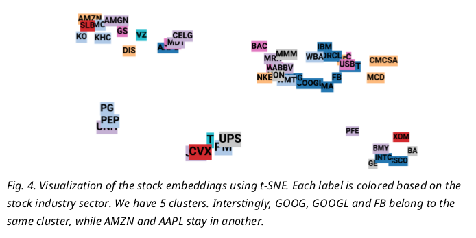
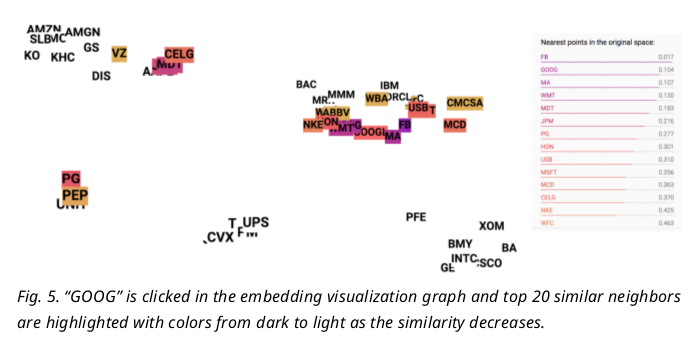
Since embedding vectors are variables to learn, Similar stocks could be associated with similar embedding and help the prediction of each others, such as “GOOG” and “GOOGL” which you will see in Fig.5.later
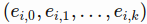
- In RNN, at one time step t, the input vector contains input_size(labelled as w) daily price values of i-th stock
- The stock symbol is uniquely mapped to a vector of length embedding_size(labelled as k),
-
As illustrated in Fig.1, the price vector is concatenated with the embedding vector and then fed into the LSTM cell
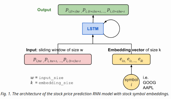
- Two new configuration settings are added into RNNConfig:
- embedding_size : controls the size of each embedding vector
- stock_count : refers to the number of unique stocks in the dataset
class RNNConfig():
   # ... old ones
   embedding_size = 3
   stock_count = 50
Define the Graph
(1) define tf.Graph() named lstm_graph and a set of tensors to hold input data. One more placeholder to define is a list of stock symbols associated with the input prices. Stock symbols have been mapped to unique integers beforehand with label encoding
# Mapped to an integer. one label refers to one stock symbol.
stock_labels = tf.placeholder(tf.int32, [None, 1])
(2) we need to set up an embedding matrix to play as a lookup table, containing the embedding vectors of all the stocks. The matrix is initialized with random numbers in the interval[-1,1] and get updated during training
# NOTE: config = RNNConfig() and it defines hyperparameters.
# Convert the integer labels to numeric embedding vectors.
embedding_matrix = tf.Variable(
    tf.random_uniform([config.stock_count, config.embedding_size], -1.0, 1.0)
)
(3) Repeat the stock labels num_steps times to match the unfolded version of RNN and the shape of inputs tensor during training. The transformation operation tf.tile receives a base tensor and creates a new tensor by replicating its certain dimensions multiple times For example, if the stock_labels is [[0],[0],[2],[1]] tiling it by [1,5] produces [[0 0 0 0 0], [0 0 0 0 0], [2 2 2 2 2], [1 1 1 1 1]]
stacked_stock_labels = tf.tile(stock_labels, multiples=[1, config.num_steps])
(4) Then we map the symbols to embedding vectors according to the lookup table embedding_matrix
# stock_label_embeds.get_shape() = (?, num_steps, embedding_size).
stock_label_embeds = tf.nn.embedding_lookup(embedding_matrix, stacked_stock_labels)
(5) Finally, combine the price values with the embedding vectors. The operation tf.concat concatenates a list of tensors along the dimension axis. In our case, we want to keep the batch size and the number of steps unchanged, but only extend the input vector of length input_size to include embedding features
# inputs.get_shape() = (?, num_steps, input_size)
# stock_label_embeds.get_shape() = (?, num_steps, embedding_size)
# inputs_with_embeds.get_shape() = (?, num_steps, input_size + embedding_size)
inputs_with_embeds = tf.concat([inputs, stock_label_embeds], axis=2)
tf.concat <= axis=2 example
Training Session
- Before feeding the data into the graph, the stock symbols should be transformed to unique integers with label encoding
from sklearn.preprocessing import LabelEncoder label_encoder = LabelEncoder() label_encoder.fit(list_of_symbols) - The train/test split ratio remains same, 90% for training and 10% for testing, for every individual stock
Visualize the Graph
-
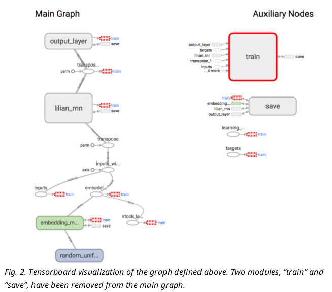
- It looks very much like our architecture illustration in Fig.1
- Tensorboard also supports embedding visualization
Results
The model is trained with top 50 stocks with largest market values in the S&P 500 index
python main.py --stock_count=50 --embed_size=3 --input_size=3 --max_epoch=50 --train

stock_count = 100
input_size = 3
embed_size = 3
num_steps = 30
lstm_size = 256
num_layers = 1
max_epoch = 50
keep_prob = 0.8
batch_size = 64
init_learning_rate = 0.05
learning_rate_decay = 0.99
init_epoch = 5
Price Prediction
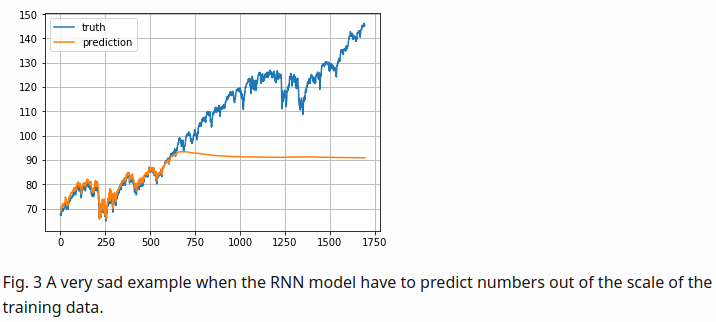
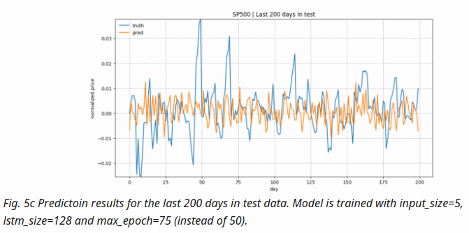
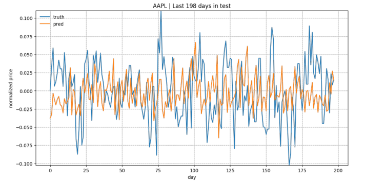
As a brief overview of the prediction quality, Fig. 3 plots the predictions for test data of “KO”, “AAPL”, “GOOG” and “NFLX”. The overall trends matched up between the true values and the predictions. Considering how the prediction task is designed, the model relies on all the historical data points to predict only next 5 ( input_size ) days. With a small input_size , the model does not need to worry about the long-term growth curve. Once we increase input_size , the prediction would be much harder
Embedding Visualization
One common technique to visualize the clusters in embedding space is t-SNE (Maaten and Hinton, 2008), which is well supported in Tensorboard. t-SNE, short for “t-Distributed Stochastic Neighbor Embedding, is a variation of Stochastic Neighbor Embedding (Hinton and Roweis, 2002), but with a modified cost function that is easier to optimize
- Similar to SNE, t-SNE first converts the high-dimensional Euclidean distances between data points into conditional probabilities that represent similarities.
- t-SNE defines a similar probability distribution over the data points in the low-dimensional space, and it minimizes the Kullback–Leibler divergence between the two distributions with respect to the locations of the points on the map
Known Problems
- The prediction values get diminished and flatten quite a lot as the training goes. That’s why I multiplied the absolute values by a constant to make the trend is more visible in Fig. 3., as I’m more curious about whether the prediction on the up-or-down direction right. However, there must be a reason for the diminishing prediction value problem. Potentially rather than using simple MSE as the loss, we can adopt another form of loss function to penalize more when the direction is predicted wrong
- The loss function decreases fast at the beginning, but it suffers from occasional value explosion (a sudden peak happens and then goes back immediately). I suspect it is related to the form of loss function too. A updated and smarter loss function might be able to resolve the issue.
Code Analysis
- first, build lstm rnn network
- second, run training
def main(config=DEFAULT_CONFIG):
  lstm_graph = build_lstm_graph_with_config(config=config)
  train_lstm_graph('SP500', lstm_graph, config=config)
build network
class RNNConfig():
    input_size = 1
    num_steps = 30
    lstm_size = 128
    num_layers = 1
    keep_prob = 0.8

    batch_size = 64
    init_learning_rate = 0.001
    learning_rate_decay = 0.99
    init_epoch = 5
    max_epoch = 50

def build_lstm_graph_with_config(config=None):
    tf.reset_default_graph()
    lstm_graph = tf.Graph()
    ...
    with lstm_graph.as_default():
        ...
        inputs = tf.placeholder(tf.float32, [None, config.num_steps, config.\
          input_size], name="inputs")
        targets = tf.placeholder(tf.float32, [None, config.input_size],\
         name="targets")
        ...
        def _create_one_cell():
          lstm_cell = tf.contrib.rnn.LSTMCell(config.lstm_size,state_is_tuple=True)
        ...
        cell = tf.contrib.rnn.MultiRNNCell([_create_one_cell() for _ \
          in range(config.num_layers)],state_is_tuple=True)
        val,_ = tf.nn.dynamic_rnn(cell,inputs,dtype=tf.float32,\
          scope="lilian_rnn")

        # Before transpose, val.get_shape() = (batch_size, num_steps, lstm_size)
        # After transpose, val.get_shape() = (num_steps, batch_size, lstm_size)
        val = tf.transpose(val, [1, 0, 2])

        with tf.name_scope("output_layer"):
            # last.get_shape() = (batch_size, lstm_size)
            last = tf.gather(val, int(val.get_shape()[0]) - 1, name="last_lstm_output")

            weight = tf.Variable(tf.truncated_normal([config.lstm_size, config.input_size]), name="lilian_weights")
            bias = tf.Variable(tf.constant(0.1, shape=[config.input_size]), name="lilian_biases")
            prediction = tf.matmul(last, weight) + bias

            tf.summary.histogram("last_lstm_output", last)
            tf.summary.histogram("weights", weight)
            tf.summary.histogram("biases", bias)
        ...
prediction.get_shape()
>> TensorShape([Dimension(None), Dimension(1)])

last.get_shape()
>> TensorShape([Dimension(None), Dimension(128)])

val.get_shape()
>> TensorShape([Dimension(30), Dimension(None), Dimension(128)])
-
Adding Jupyter Notebook path, tf.transpose , tf.gather example, tensor example
tensor example
# https://www.tensorflow.org/api_guides/python/array_ops
import tensorflow as tf
import numpy as np
import pprint
tf.set_random_seed(777)  # for reproducibility

pp = pprint.PrettyPrinter(indent=4)
sess = tf.InteractiveSession()

t = tf.constant([1,2,3,4])
print(tf.shape(t).eval())
print(t.eval())

>> [4]
>> [1 2 3 4]

t = tf.constant([[1,2,3,4]])
print(tf.shape(t).eval())
print(t.eval())
>> [1 4]
>> [[1 2 3 4]]

x = [1, 4]
y = [2, 5]
z = [3, 6]

# Pack along first dim.
tarr = tf.stack([x, y, z],0).eval()

tarr
>> array([[1, 4],
       [2, 5],
       [3, 6]], dtype=int32)

tarr = tf.gather(tarr,[2,0])
# tf.shape(tarr).eval()
tarr.eval()

>> array([[3, 6],
       [1, 4]], dtype=int32)

t = np.array([[[0, 1, 2], [3, 4, 5]], [[6, 7, 8], [9, 10, 11]]])
pp.pprint(t.shape)
pp.pprint(t)

>> (2, 2, 3)
array([[[ 0,  1,  2],
        [ 3,  4,  5]],

       [[ 6,  7,  8],
        [ 9, 10, 11]]])

t1 = tf.transpose(t, [2, 1,0])
pp.pprint(sess.run(t1).shape)
pp.pprint(sess.run(t1))

>> (3, 2, 2)
array([[[ 0,  6],
        [ 3,  9]],

       [[ 1,  7],
        [ 4, 10]],

       [[ 2,  8],
        [ 5, 11]]])

t1.get_shape()[0]
>> Dimension(3)

last = tf.gather(t1,int(t1.get_shape()[0])-1,name="test_output")

last
>> <tf.Tensor 'test_output:0' shape=(2, 2) dtype=int64>

pp.pprint(sess.run(last).shape)
pp.pprint(sess.run(last))

>> (2, 2)
array([[ 2,  8],
       [ 5, 11]])